Annals of Mathematics and Physics
Waves of the dynamics of the rate of increase in the parameters of Covid-19 in Russia for 03/25/2020-12/31/2020 and the forecast of all cases until 08/31/2021
Mazurkin PM*
Cite this as
Mazurkin PM (2021) Waves of the dynamics of the rate of increase in the parameters of Covid-19 in Russia for 03/25/2020-12/31/2020 and the forecast of all cases until 08/31/2021. Ann Math Phys 4(1): 048-065. DOI: 10.17352/amp.000024In applied mathematics and statistics, only linear equations are still used. The article proposes the sum of asymmetric wavelets with variable amplitudes and periods of oscillation. As a result, the behavior of any object or subject is given by the sum of vibrations. Using the identification method based on statistical daily data on four indicators of the dynamics of the rate of Covid-19, quanta of the pandemic behavior in the territory of the Russian Federation from March 25 to December 31, 2020 were identified. It is shown that the rates are infected, cured, died, and “all cases = infected + cured + died” in Russia got two superimposed bulges. Based on the computational capabilities of CurveExpert-1.40, 4-5 components were jointly identified with an overall correlation coefficient above 0.86 for infected and over 0.99 for all cases. It has been proven that the spread of the virus has the form of a set of finite-dimensional wavelets with variable amplitudes and, as a rule, with a decreasing oscillation period. By modeling the standard deviation by the serial numbers of the wavelets, it was proved that the parameters of the Covid-19 pandemic have fractal distributions. For the velocity parameter “died”, the main bulge does not reach its maximum. And the second member of the trend peaked at 164 deaths on 06/18/2020, and it will leave the scene from 03/23/2021. The third member of the model, aimed at countering mortality, at the beginning of the time series on 03/25/2020 received a fluctuation period of 355 days. By the date of December 31, 2020, the fluctuation period became equal to 278 days. More often with constant half-periods of 3.5 and 16.1 days, fluctuations occurred. In this case, the 70th term gives a constant oscillation period, even 1.88 days. The average relative modeling error in modulus is equal for speeds: 1) died - 2.09; all cases - 3.22; cured - 17.17 and infected 29.91%. In this case, the range of error values changes in the following intervals: 1) died from -18.93 to 11.95%; all cases from -31.37 to 20.20%; cured from -248.8 to 396.0%; infected from -1934.0 to 779.7%. According to the distributions of the relative error after 1%, the following rating was obtained: 1) the correlation coefficient of 0.9807 for the speed died; 2) at 0.9768 the rate of all cases; 3) 0.8640 has been cured; 4) 0.8174 - infected. The fractality coefficient is equal to the ratio of the standard deviations of the linear model to the last component: for infected 3572.76 / 310.97 = 11.5; cured 5.8; died 24.3 and all cases 9.6. Further, due to the high range of relative error, the rates of cured and infected are excluded from forecasting. The forecast for the rate of deaths was carried out until 02/14/2021. The right border at the forecast horizon was adopted due to the fact that negative values appear from 15.02.2021. For a longer time interval from 01.01.2021 to 31.08.2021 the model allows predicting the rate of change of all cases. To reduce the relative modeling error, it is recommended to re-identify the model of the dynamics of the parameters died and all cases every three weeks. The identification method is applicable to any statistical series, and not only to dynamic ones.
Introduction
For the readers of the Annals of Mathematics and Physics journal, this article proposes a method for identifying asymmetric wavelet signals using a specific example of dynamic daily series of parameters of the Covid-19 pandemic in Russia. The mathematical formulation of identification is based on the concept of oscillatory adaptation of phenomena and processes in nature. Including in real time, there are strong fluctuations between the disease of the population of Russia and the activity of populations of Covil-19 viruses. As a result, the daily publication of statistical data allowed us to outline the methodology for identifying asymmetric wavelets [1-3]. Study guides have been published for students.
Nature’s third report on the progress of the pandemic, coming out at the end of the first year of the pandemic, contains key epidemiological findings, from early warning to tracking the effects of new variants [4].
This editorial [4] further notes that epidemiology itself is expanding with the involvement of researchers from other fields, such as physics, mathematics, computer science and network sciences, who contribute to the development of their ideas and knowledge. The US government announced the creation of the National Center for Epidemic Forecasting and Outbreak Analysis. We hope this will be the epidemiological equivalent of the Central Meteorological Office, an independent body that provides forecasts using the most advanced computing power and the best available data.
The purpose of the article is to use the example of time series from March 25 to December 31, 2020 to conduct a wavelet analysis and identify the quanta of behavior of the ergatic system “Covid-19 + Russian health care system” based on the speed dynamics of four pandemic parameters (infected, cured, died, cases = infected + cured + died), then the formation of a forecast model and verification according to data from January 1 to January 25, 2021.
Epidemiologists predicting the spread of Covid-19 must use climate modeling techniques to make predictions more reliable, say computer scientists, who have spent months auditing one of the most influential pandemic models [5]. In this article, we have applied the method of wavelet analysis from quantum meteorology [6] to identify the sum of solitary waves in the process of pandemic behavior.
Further David Adam notes the following [7]. Many of the disease models are unique to the individual academic groups that have developed them over the years. But the mathematical principles are similar. They are based on attempts to understand how people move between three main conditions and how quickly: people are either susceptible to the virus; got infected (I); and then either recover (R) or die. It is assumed that the R group is immune to the virus, so it can no longer transmit infection. People with natural immunity would also belong to this group [7].
For the first three months of 2020, according to statistical data, a dynamic epidemiological model was proposed to recognize the initial stage of Covid-19 infection among countries in the modern world [8]. The article [9] also notes that the epidemiological curves show an exponential relationship of growth.
Such exponential models are applied not only in epidemiology. For example, to study the dynamics of the distribution of investment schemes in this population, an epidemiological model was created, in which the rate is included in the model as an exponentially distributed random variable that gives distribution of losses [10].
Based on the concept of vibrational adaptation in nature and the use of trigonometric sums [11] of the cosine, a method of sequential identification [1] of the general formula for an asymmetric wavelet signal was proposed to obtain a set in the form of a sum of stable wave patterns from tables of quantitative data, especially from tables of statistical data [2] in time.
Then each component of the trigonometric sum is a wavelet signal, and each wavelet in the CurveExpert-1.40 software environment is constructed from the so-called Hilbert bricks [2]. As a result, from such general invariants in the form of wavelets, a polynomial algebraic equation is constructed, sometimes containing more than 200 wavelets. Thus, we have proved the possibility of forming one single algebraic equation according to Descartes directly without solving differential and integral equations.
Thus, we do not address the detailed epidemiological reasons for the formation of statistical time series. For wavelet analysis, the data is accepted as it is, that is, without any consideration of measurement errors. Moreover, no grouping of data is allowed. The quality factor of the initial data is checked as follows: the more wavelets the dynamic series will be decomposed with the minimum value of the maximum relative error of the residuals (the difference between the fact of measurements and the calculation by formulas) after the last fluctuation, the higher the quality of the initial tabular data. With an increase in the length of the dynamic series, the set of wavelets also increases, but there is a possibility of lengthening the forecast horizon for the future.
The proposed identification method made it possible, for example, to carry out a wavelet analysis up to the measurement error of the maximum temperature in Central England [12]. Each component of the trigonometric sum is a quantized signal about the behavior of the object of study, for example, in the article [6] in quantum meteorology about the behavior of the temperature of the surface air layer.
Materials and methods
Initial data
Table 1 shows a fragment of daily data from the site https:// стопкоронавирус.рф/information/. The origin of coordinates on the abscissa axis is taken for the date 03/25/2020, and for four time series, the end is December 31, 2020.
In table 1, the following conventions are adopted, person/day: SI – Speed infected; Scu– Speed cured; SD – Speed died; Sca – The speed or pace of daily occurrences.
Identification method
The process of identifying stable patterns is presented as a sequential process of solving the problem of statistical (probabilistic) modeling by asymmetric wavelet signals based on dynamic and other series of measurements. The problem of the development of methods of the calculus of variations (Hilbert’s 23rd problem) has not yet been solved, although much has been done in this direction of mathematics by Hilbert himself [1-3,6,12].
The key to the understanding by classical mathematicians of the proposed methodology for identifying invariants by real algebraic number fields, as the results of multivariate physical measurements, is the heuristic statement: “The guiding principle for Hilbert was the analogy with the corresponding problems for algebraic functions in one variable” [1].
Identification by tabular data (numeric field) includes the following stages:
1) Heuristic identification of the essence of the phenomenon or process under study based on the results of measurements and analysis of the tabular model (a priori information) and comprehension in the course of identifying a structure in a statistical one-factor pattern by its additive components (a posteriori information);
2) Structural identification of each one-factor mathematical function in the general model as a sum of invariants from asymmetric wavelet signals;
3) Parametric identification of a stable pattern, which is built up according to individual invariants, in the form of an asymmetric wavelet in the CurveExpert-1.40 software environment.
The criterion (quantitative measure) of the identification process is the measurement error when compiling a numerical field, i.e. source data tables. For example, prime numbers and their series do not have a measurement error: they are absolutely solid and reliable. Other types of data have different errors. Thus, mathematical number objects are the best for identifying invariant laws.
In second place are precision measurements in astronomy, physics, engineering and technology, and other fields of science and technology.
The third place is taken by biological objects, and their behavior has a clearly manifested oscillatory character, therefore, linear and linearized models are generally not suitable for biologists.
The highest errors have socio-economic measurements due to their high subjectivity of meaningful ideas about the behavior of natural, natural-anthropogenic and anthropogenic objects.
We have long abandoned approximation methods and, accordingly, do not use statistics programs from Excel at all. In identification, the first stage (variation of functions) is excluded from the theory of approximation - stable laws are predefined as invariants. From them, as from bricks, various mathematical constructs are created.
Thus, at the heuristic level, Hilbert’s 23rd problem has not yet been sufficiently formalized by us. But it was completely solved at the structural and parametric levels of analysis and synthesis. The variation of functions is reduced to a conscious selection of stable laws and the construction on their basis of adequate stable wave patterns. In the future, it is planned to automate the construction of one-factor models for any tabular data (numerical matrices) based on multifactor measurements. But for this we need to create a special software environment according to our scripts.
Wavelet analysis and identification technology
General wavelet formula: We adhere to Descartes’ concept of the need for direct application of the general algebraic equation as the final mathematical solution of unknown integral equations. Generalizing many examples, including in the form of a list (space) of objects located in the same time section, we proposed a new class of wave functions [1].
Any time series, in particular the annual temperatures in Central England, is understood as a series of signals in the form of asymmetric bursts. Time is taken from the beginning of the forecast base from 1878 [12]. Then we get the positive direction of the abscissa axis.
In this case, each wavelet becomes a separate quantum of behavior, and many quanta form a kind of beam of various oscillations with variable amplitude and period. A set of wavelets forms the residuals from the actual values of the time series (absolute error). If it is less in comparison with the measurement error, then it is argued that the dynamic temperature series has a high quantum certainty (within the measurement error).
Wavelet signal, as a rule, of any nature (object of study) is mathematically recorded by the wave formula [1] of the form
, , , (1)
where y – the index (dependent factor), i– the number part of the model (1), m– is the number of terms in the model (1), in our case equal to 64, x– is the explanatory variable (influencing factor), a1…a8– the parameters of the model that accepts numeric values in the course of structural-parametric identification in the software environment CurveExpert-1.40 (URL: http://www.curveexpert.net/), Ai – the amplitude (half) of wavelet (axis y), Pi – half-period fluctuations (axis x).
Quantum of behavior as a signal
According to the formula (1) with two fundamental physical constants e (the number of Neper or the number of time) and π (the number of Archimedes or the number of space), a quantized wavelet signal is formed from within the studied phenomenon and/or process. The concept of wavelet signal allows us to abstract from the physical meaning of many statistical series of measurements and consider their additive decomposition into components in the form of a sum of individual wavelets.
A signal is a material carrier of information. Temperature appears as an energetic consequence of air currents in the surface air layer. Of the many definitions, we understand information as a measure of interaction between material carriers.
The signal can always be generated, but its reception by a person is not required. For example, the average annual temperature in Central England has been known since 1659, but until now, as a bunch of signals in the form of asymmetric bursts, this dynamic series for 360 years has not been deciphered. For the maximum temperature [3], the same heuristic is required.
Any physical process or part of it can be a signal. It turns out that the change in the set of unknown signals has long been known by measurement methods, for example, in the form of temperature series, and at many meteorological stations. However, there are still no statistical models of the dynamics of weather and climatic parameters at each meteorological station.
Three types of wavelets
Under the conditions and in formula (1), we obtain three types of asymmetric wavelets:
1) Finite-dimensional wavelet: at the amplitude from formula (1), according to the biotechnical law [4] , according to the condition , a wavelet is formed, which has left and right boundaries of the variable value interval on the positive abscissa axis x;
2) Infinite-dimensional wavelet: according to the condition for the amplitude from formula (1) , we obtain an asymmetric wavelet that has no boundaries, and it is our modified Mandelbrot’s law in physics under the condition (Laplace’s law in mathematics, Zipf-Pearl in biology, Pareto in econometrics) has an infinite semi-axis of abscissas, starting from zero;
3) under the condition , an abnormal asymmetric wavelet is formed, when the power function turns into a power law that has no physical meaning, therefore, the identification process continues further on passing from a finite-dimensional wavelet to an infinite-dimensional one.
Only the first two types of wavelets are used in the identification process.
Comparison of quanta of pandemic and temperature behavior
In this article, we confirm the conclusion of David Adam that climate modeling methods should be used to predict the spread in time of Covid-19 [5]. However, the wavelet analysis of behavior invariants from quantum meteorology [6] showed that almost half of the components in the general model (1) contain infinite-dimensional oscillations.
At the same time, all four parameters of Covid-19 in Russia gave the sums of trigonometric equations, all of which are finite-dimensional equations. Hence, the first conclusion suggests itself that the dynamics of the pandemic are not affected by space and climatic cycles. The second finding is that the parameters of Covid-19 appear to be seasonal (monthly cycles).
Apparently, the influence of cycles with a frequency of several years is possible, for example, the influence of a two-year cycle of plant productivity. To prove such cycles, data on the dynamic series of the pandemic over several years are needed. So far, we can only conclude that Covid-19 is a phenomenon accompanying the behavior of people in various countries.
Non-linear trend
Such a trend is formed from equation (1) when the oscillation period tends to infinity, that is, under the condition . A special case is the condition under which the measurement period is many times less than the oscillation period of the studied process.
For the climatic factor of air temperature, due to the influence of space and climatic cycles in the general trigonometric formula, for example, according to the average annual temperature of Central England since 1659 (the measurement cycle is more than 360 years), 188 wavelets were obtained, of which a considerable part belong to infinite-dimensional vibrations. For such long series of dynamics, the main trend is Mandelbrot’s law.
For short time series of temperature, a trend was obtained from two components of the form
. (2)
Here, for various natural and natural-anthropogenic processes, the first term of the trend is the modified Mandelbrot’s law, and the second term is the biotechnical law [1].
For the dynamics of the Covid-19 parameters over 282 days, when only finite-dimensional wavelets are present in the general algebraic formula, a trend of the form was obtained
, (3)
где – the parameters of the model (3) that accepts numeric values in the course of structural-parametric identification in the software environment CurveExpert-1.40 (URL: http://www.curveexpert.net/).
First, the first term is identified, showing the second hump of the change in the values of the Covid-19 parameters, while having a greater length in time compared to the first bulge. Then the parameters of model (3) are sought for both convexities.
Identification of the trend
To identify formulas (2) and (3), several textbooks for students have been published in Russian.
Identification technology based on the principle from simple to complex, for any data pairs in the CurveExpert-1.40 software environment is reduced to the following procedures:
1) In most cases of modeling, the process of identifying quanta of behavior in the form of nonlinear equations begins with a linear model;
2) Then sequentially complicating the linear model to construct a mathematical expression (2) or (3), we obtain the trend equation;
3) If the residuals on the trend graph clearly show the location of the points in the form of fluctuations, then proceed to the identification of the wavelet (1).
Wave equation identification (1)
Students begin to master the method of identifying simple patterns such as Mandelbrot’s law from the second year of the bachelor’s degree, and some students identify the parameters of model (1) in the master’s degree.
To identify formula (1), we have published two teaching guides for students. There are only scientific articles on modeling the time series of air temperature and the content of pollutants, and even more so the parameters of Covid-19.
When identifying a set of wavelets in a temperature series, we found that the length of the data series significantly affects the transition from the trend to the first oscillation. When the duration of the temperature series exceeds 175 years, a complex relationship arises between the first components of the general formula (1).
The technology for identifying formula (1) according to the principle from simple to complex includes the following basic procedures:
1) For an infinite-dimensional wavelet, the simplest wave equation is identified , and for a finite-dimensional wavelet, the identification process begins with a simplified formula (the initial values of the model parameters before the first step are taken by the fitting method);
2) Then, by successive complication, the model is reduced to formula (1);
3) =The identification of new wavelets continues in this way until the simulation error becomes less than the measurement error, or the identification process stops earlier due to the quantum uncertainty of the behavior of the research object.
The identification process in CurveExpert-1.40 environment is laborious. Therefore, according to our scenarios, we need to create a specialized software environment for partial automation of the identification process. This will make it possible to search for wavelets with a measure of adequacy in terms of the correlation coefficient much less than 0.05.
Results of the wavelet analysis of the dynamics in Russia of the parameters of Covid-19
Velocity dynamics models
After structural-parametric identification of formulas (3) and (1), the parameters of the obtained models of the velocity dynamics for the four parameters of Covid-19 in the Russian Federation are given in Table 2.
The constant component, for example, for the infected speed equal to 154, shows the history of the indicator dynamics until March 25, 2020. As you know, in Russia, measures to counter the pandemic began actively from the beginning of March.
Before reaching the level of quantum certainty (with the appearance of difficulties in identifying the model), the components (1) were identified in the amount, pieces: Speed infected – 57; Speed cured – 15; Speed died – 70; Speed of all cases – 8.
The nature of the influence of time on the parameters of Covid-19 is determined by the sign in front of the component. A positive sign in front of the amplitude of the parameter infected shows the influence of time on the growth of the pandemic (unfavorable for humans), and a negative sign - on a decrease (favorable for humans). Then, from the data in Table 2, it turns out that the components No. 2, No. 5 and No. 57 have a negative character for the infected speed for people. Likewise, for speed has died a positive meaning for people gets a negative sign for members # 3, # 5 and # 70.
The opposite direction in meaning gets the speed parameter cured. Here, a positive sign becomes positive for humans, and a negative sign becomes positive for the Covid-19 pandemic. In this regard, the first five members from Table 2 are aimed at increasing those who have been cured, and the last component No. 15 shows some shortcomings of specialists due to an increase in the activity of the virus.
Half the amplitude for finite-dimensional wavelets is a bio-technical law [1], which shows the simultaneous influence of two forces. The first force changes according to a power function , and the second - according to our modified Mandelbrot’s law .
However, for modeling a pandemic, a case arises when the third parameter of model (1) changes sign and half of the amplitude receives a formula of the form , which we called the anomalous law of double growth. This, as a rule, is obtained due to the fact that the dynamic statistical series has not received the convexity limit and therefore both forces become laws of growth (the first component in the form of a power function, and the second - in the form of an exponential growth law).
Speed infected SI
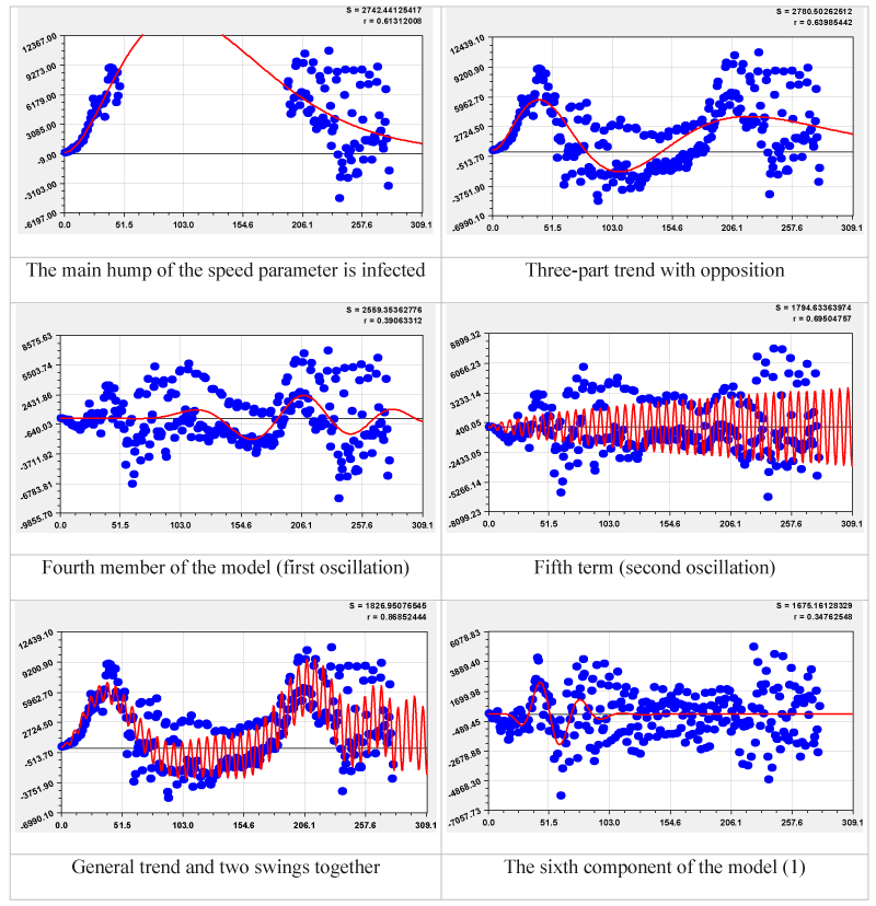
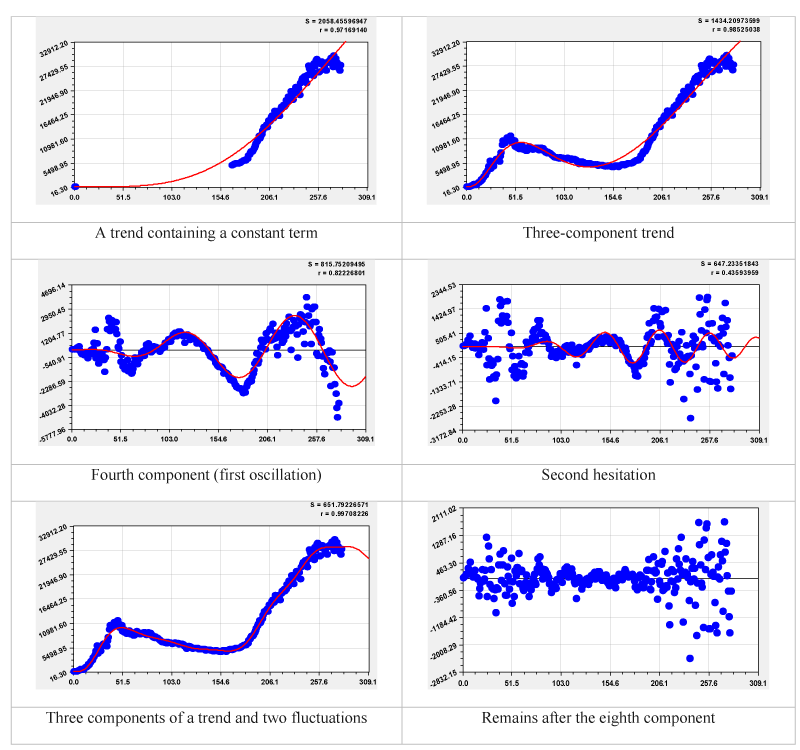
For speed infected, the first three terms form a trend (Figure 1). The first member is a permanent number of 154 people. This value shows the prehistory of the pandemic in Russia before March 25, 2020. The second component shows the main bulge, which reached its maximum on 06/07/2020. The third term of the trend, due to the negative sign, displays the inverse bulge of the infected velocity dynamics graph. As a result, this member shows good opposition of the Russian health care system to the growth of the Covid-19 pandemic.
Further, 54 more components were revealed in the form of solitary waves of oscillatory disturbance. At the same time, the fourth component received a negative sign and shows the counteraction of physicians with a variable oscillation period. On the date of 25.03.2020, the oscillation period was 187.27945 2 375 days. This was the first and very slow reaction in Russia to the rate of infected. Then the wave becomes more frequent and on 31.12.2020 the period of oscillation for the fourth component is reduced to 109 days with an increase in the oscillation frequency by 3.4 times.
The fifth term with a positive sign indicates the quantum of Covid-19 behavior. On 03/25/2020, the period of fluctuation in the speed of the infected was 3.51286 2 7 days. At the beginning of our registration of a pandemic in Russia on 03/25/2020, the rate of spread of infected people is 375/7 = 53.6 times higher than the oscillatory indignation of the healthcare system. Due to the opposition of doctors, the weekly cycle of virus outrage was reduced by the end of the year to a half-period of 3.50963 days. For 282 days, the period of fluctuation of the infected in this quantum of behavior decreased slightly. The increase in the vibration frequency was only 3.51286 / 3.50963 = 1.00092 times. This means that the spread of the virus is always almost stable.
With a constant period, as, for example, in quanta of behavior # 6 and # 7, 28 wavelets were identified, which is 100 28/57 49.12% of their total number.
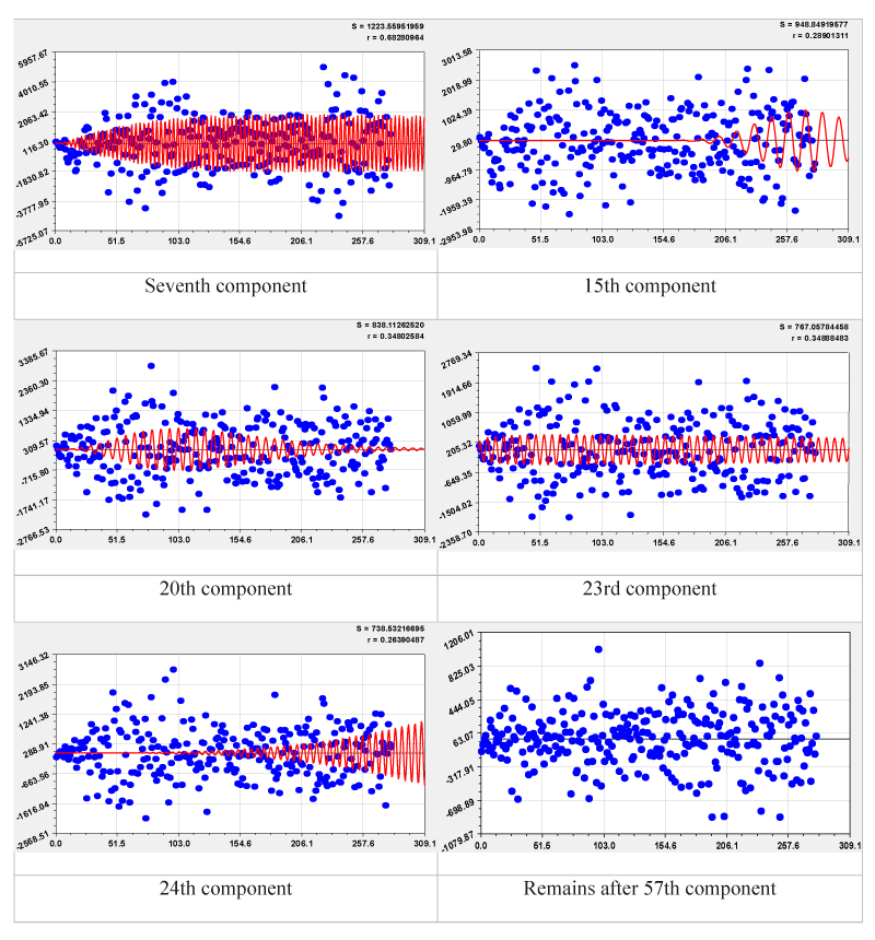
The rest of the characteristic terms from Table 2 are shown in Figure 2.
According to the computing capabilities of the CurveExpert-1.40 software environment, five components were jointly identified. Each wavelet was further revealed separately from the first five members. As can be seen from the graphs in Figure 1, the finite-dimensional fourth and fifth terms affect the future, the fifth oscillation gives a small dying influence, and the sixth component was in the past time in the spring of 2020. Therefore, such wavelets are not involved in the compilation of the predictive model.
In Figure 2, the seventh component has a length since the beginning of registration on March 25, 2020 and will continue far into the future. Similarly, a long wave is formed along the 23rd component. Short-term wavelet # 15 started in mid-October and will not last long, and wavelet # 24 is dangerous because of the future growth of the oscillation amplitude. At the same time, wavelet # 20 is a thing of the past. The residuals after the 57th component were used to calculate the modeling error.
Speed cured SCu
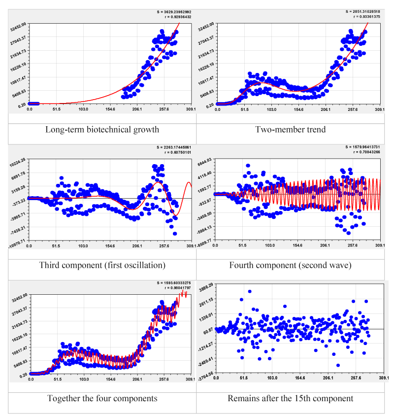
The composite trend receives the sum of two biotechnical laws (Table 2) according to the first type of finite-dimensional wavelets with an oscillation period tending to infinity (Figure 3). Speed cured is a result of the behavior of the Russian healthcare system. It is directed against the behavior of Covid-19 among the population.
The first component of the trend (main bulge) does not reach its maximum in the first half of 2021. And the second term of the trend reached a maximum of 6356 cured on 06/08/2020, and he left the scene of the speed dynamics cured from about 12/28/2020. The third component as of 03/25/2020 received an oscillation period of 350.15841 2 700 days. This means that the Russian healthcare system began to be deployed only in March 2020. By the date of December 31, 2020, the oscillation period became equal to 50.03086 2 100 days.
Thus, the oscillatory adaptation of doctors in Russia to the treatment of the population from Covid-19 has increased sevenfold in 282 days. Much more often with constant half-periods of 3.5 and 3.7 days, fluctuations of the cured occurred with an almost weekly frequency.
Speed died SD
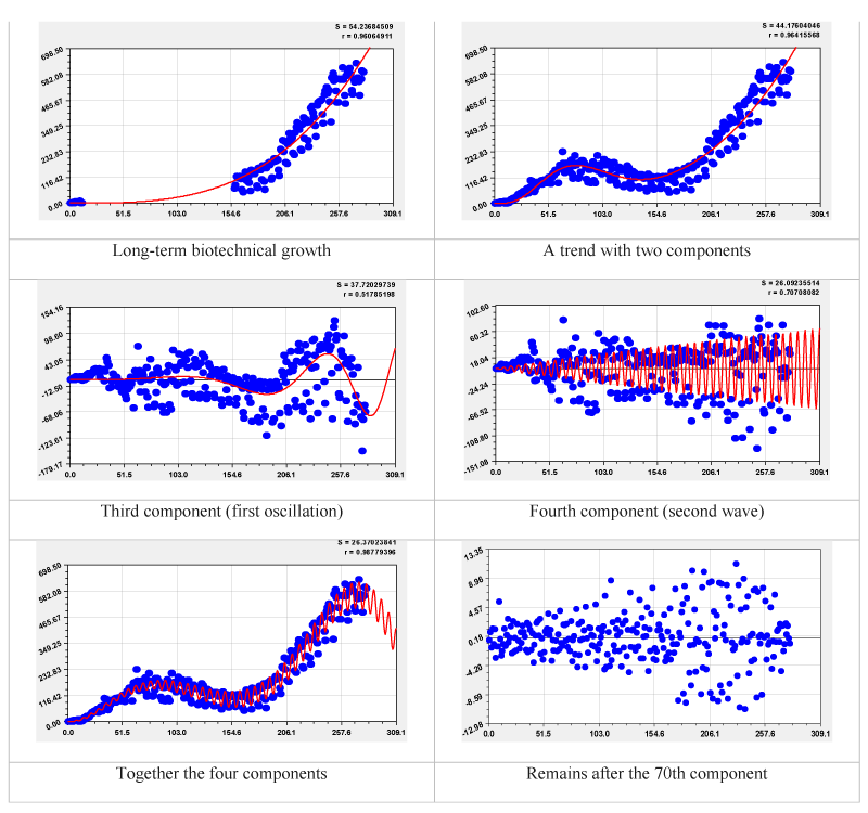
The general trigonometric equation received 70 components. The nature of the equations and trend graphs (Figure 4) is similar to the previous parameter.
As with the previous parameter, the first term in the trend (the main bulge) does not reach its maximum quickly. And the second component of the trend has already reached a maximum of 164 deaths as of 06/18/2020, and it will disappear from the scene of the speed dynamics died approximately from 03/23/2021. The third component, aimed at countering mortality, as of March 25, 2020, received a fluctuation period of 177.64868 2 355 days. By the date of December 31, 2020, the fluctuation period became equal to 139.2171 2 278 days.
Then, the oscillatory adaptation of physicians in Russia to the fight against mortality from Covid-19 increased only 1.28 times. More often, with constant half-periods of 3.5 and 16.1 days, fluctuations in the parameter pandemic died. In this case, the 70th term gives a constant oscillation period, even 1.88 days.
Speed of all cases SCa
Together with the permanent member, only eight components were received. The graphs of the components and the distribution of residues after the eighth component are shown in Figure 5.
From the residuals in Figures 4,5, it can be seen that the spread of values has increased since autumn 2020, that is, the pandemic spreads seasonally (two bulges in the location of points in the residuals after the eighth component in Figure 5). As a result, the data on Covid-19 gets the character of a scedastic distribution, rather than a uniform one.
According to the computational capabilities of CurveExpert-1.40, it was found that the parameter of all cases receives the greatest adequacy with a correlation coefficient of 0.9971, in the second place with a correlation coefficient of 0.9878 is the speed died, in the third place - the speed is cured and in the fourth place - the speed is infected.
Discussion of the results of identification of wavelet signals
Quantization of behavior
In nature, there are quanta of state (structure) and quanta of behavior (functioning). Quantums of state are known in the quantum physics of elementary particles. However, structure quanta also exist for macro-objects, for example, quantization of a state occurs in crystals and rock crystalline formations. Therefore, quantum physics of state exists for macro-objects as well.
Behavioral quanta are inherent in living matter (a term according to V.I.Vernadsky) and functioning quanta refer to inert matter repeatedly processed in the Universe by living matter, including technical means created by living organisms, including humans.
Systems involving a person are called ergatic. Then the Covid-19 pandemic, spreading among people of all countries of the world, has clear distributions according to the parameters of quanta of behavior in the form of wavelet signals. But, first of all, due to errors in measurements (measurement is quantization by units of measurement), the identification of wavelets is possible up to a certain level on the border between the possibility and impossibility of quantizing the behavior process.
Moreover, this border in this article is taken up to the level of the correlation coefficient of 0.05. If the wavelets receive an adequacy less than 0.05, then we stopped the process of identifying this wavelet. Using a special software environment created according to our scenarios, of course, you can significantly lower the quantization limit. But then the number of terms in the general formula (1) will increase.
As a result, we distinguish two types of quantization of the behavior of the system under study:
firstly, in dynamics, each factor is divided into a sum of wavelets, that is, in time, the factor is represented as a bundle of solitary waves (solitons) and this process is characterized as quantum certainty in the process of behavior (this mainly refers to meteorological and geomorphological parameters having a fairly small error in measurements);
Second, the set of residuals from the first case in terms of the relative modeling error receives quantum uncertainty in the behavior of the system.
As a rule, the quantum uncertainty reaches no higher than the trend level, when it is impossible to identify the wave components, for binary relations between meteorological and other parameters.
Thus, any phenomenon or process can be assessed according to the level of adequacy of the general model (1) (there is no connection at the correlation coefficient , weak coupling at , medium coupling at , strong coupling at , strongest coupling at , superstrong coupling at ) decomposition of the functional connectivity of the system into quantum certainty and quantum uncertainty. In this case, quantum certainty is estimated by the correlation coefficient, and uncertainty - by the difference.
Modeling errors
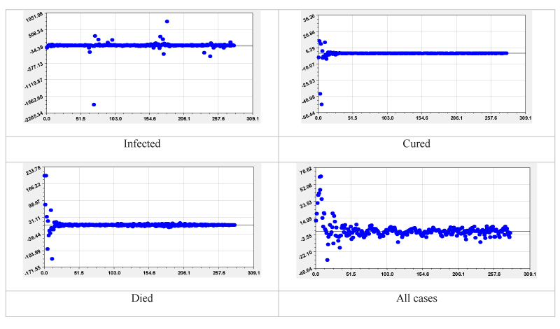
The graphs of the relative error for all four time series without their truncation are shown in Figure 6. The graph of the relative error in infected shows the presence of sharply deviating points, which indicates negligence in recording some values of the pandemic parameter.
The other three parameters received high values of relative error at the beginning of the series, which indicates instability in the behavior of the Russian healthcare system at the beginning of the response to the Covid-19 pandemic.
For modeling, you need to cut off the chaotic origin for all four parameters. It turned out that for the Russian Federation, stable trends in the dynamics of Covid-19 parameters were observed from 04/07/2020 (Table 3).
The relative error Δ was obtained by dividing the residuals (absolute error ε) after the last component of the model from Table 2 by the actual values of the Covid-19 parameters from Table 1 (multiplied by 100 to obtain a percentage). As a result, truncated time series of the speed of parameters were formed, including 269 days in terms of the relative error for the last component in the models from Table 2.
The average relative error in absolute value was calculated by the formula
(4)
The average relative modeling error in modulus is equal for the speed of the parameters: 1) died - 2.09%; all cases - 3.22; cured - 17.17% and infected 29.91%. In this case, the range of error values among 269 values varies in the following intervals: 1) died from -18.93 to 11.95%; all cases from -31.37 to 20.20%; cured from -248.8 to 396.0%; infected from -1934.0 to 779.7%. In environmental studies, it is allowed to change the relative modeling error up to 30%. Within these limits, consider the law of normal distribution (Gauss’s law).
Gauss’s law in error distributions
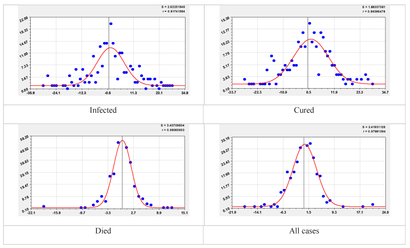
The graphs are given in Figure 7. For infected, 31 measurement points were excluded from the dynamic range. Then the statistical representativeness of the series is 100 (269 - 31) / 269 = 88.48%. The same representativeness is obtained by the number of relative errors of the parameter cured. For a number of dead and a number of all cases, all 269 measurements are within 30%.
After identifying the Gauss law, the following equations were obtained:
– The distribution of the relative error is infected (correlation 0.8174)
(5)
– The distribution of the number is cured at an interval of 1% relative error (0.8640)
(6)
– The distribution of the number died at an interval of 1% relative error (0.9807)
(7)
– Distribution of the number of all cases of relative error (0.9768)
(8)
According to the distributions of the relative error at intervals of 1% according to the graphs in Figure 7, a rating score was obtained: 1) the correlation coefficient of 0.9807 for the speed died; 2) at 0.9768 the rate is all cases; 3) 0.8640 has been cured for the speed parameter; 4) 0.8174 at the speed of dianmic is infected.
Fractal distribution of wavelets
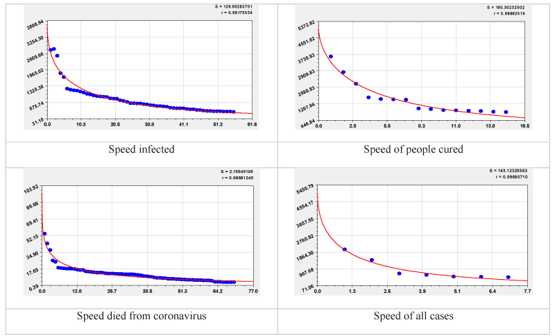
The arithmetic mean for the rate of the pandemic is not modeled, therefore the zero rank was adopted for the linear model of the type (Table 4). Further, regularities of the distribution of the standard deviation were revealed depending on the serial numbers of the components.
The indicator of the fractal distribution is the standard deviation value, which is shown in the upper right corner of the graphs. In this case, the constant term is not taken into account here, since it is not a Mandelbrot fractal. The largest series of 70 members was formed for the wavelet analysis of the velocity parameter died.
The fractality coefficient was adopted by Mandelbrot equal to 2. However, in nature, apparently, such an ideal multiplicity does not exist. As a rule, all relationships between the levels of fractals according to Table 4 are non-multiple. As can be seen from the data in Table 4, the linear model gives the standard deviation of rates, person/day: infected 3572.76; cured 4962.32; died 94.827 and all cases 5002.48. Then the coefficient of total fractality will be equal to the ratio of the standard deviation of the linear model to the standard deviation of the last component, that is, to the border of quantum uncertainty. This general coefficient of fractality will be equal to: for the parameter infected 3572.76 / 310.97 = 11.5; cured 5.8; died 24.3 and all cases 9.6.
After identification of the modified Mandelbrot’s law, the distribution patterns of the components by standard deviation were obtained (Figure 8):
– For speed infected (correlation coefficient 0.9818)
; (9)
– For the speed of people who healed (0.9886)
; (10)
– For speed died (0.9868)
; (11)
– For the speed of all cases (0.9969)
(12)
The correlation coefficient of the fractal distribution of wavelets exceeds 0.98. This fact proves that the trigonometric general equation (1) receives a strong fractal distribution of its components. All quanta of behavior in terms of the rate of daily growth in the number of infected, cured, dead, and all cases are distributed in the form of non-multiple fractals.
Forecasting Covid-19 in Russia
It is considered that an approximate forecast is possible for the forecast horizon equal to the forecast base. However, over time, already in the near future after the right border of the forecast base, new and even unknown wavelets appear, therefore the verification process based on new actual data for the Covid-19 parameters will show a tendency of discrepancy between the forecast model and the actual range of values. This comparison allows us to establish the frequency of repeated identifications in iterations.
Due to the high magnitude of the relative error, we exclude the parameters of the rate cured and infected from the forecasting process. The range of error values among 269 values varies in the intervals: 1) died from -18.93 to 11.95%; all cases from -31.37 to 20.20%.
Drawing up a forecast model
The wavelet forecasting method consists in selecting from the entire set of model members (1) those components that affect the future. Of the 70 members of the model (1), the speed died, 35 components affect the future, that is, 50% of their total number. For speed, all cases of eight terms, the second term of the trend has no effect on the future, so only seven components are taken into account in the forecast model.
Calculations of the parameters of the pandemic for the future
The parameters of the model with five significant digits given in Table 2 turned out to be insufficient in direct calculations. In this regard, all 11 significant digits were accepted, for example, the sixth term of the speed died:
User-Defined Model: y=-a*x^b*exp(-c*x^d)*cos(pi*x/e-f)
Coefficient Data:
a = 3.30280799707E-002
b = 1.56670184720E+000
c = 1.04112544062E-002
d = 9.42242065411E-001
e = 1.75181448512E+000
f = 1.68365585957E+000
The calculation was performed on columns O, P, Q of the Excel-16 software environment, and the parameters of the above wavelet model are located on column P along lines 2-7. For the 12th line of the first speed value, it died on 03/25/2020, the following entries were made:
A4 =-$P$2*B12^$P$3*EXP (-$P$4*B12^$P$5);
p4 =$P$6;
y6 =O12*COS (ПИ ()*B12/P12-$P$7).
Column B from line 12 contains 281 actually measured time values of the measurement date, and then this column was continued until for the date 02/14/2021. With a further increase in time, negative values appear in the number of deaths.
The speed died for 07/04/2020-14/02/2021
The forecast was carried out before 02.14.2021, that is, for 44 days from 01.01.2021, which is a share of 44/269 = 0.1636 of the length of the forecast base, that is, the forecast horizon will be equal to more than one sixth of the forecast base. Such a right border of the forecast horizon was adopted due to the fact that from 15.02.2021 negative values of the velocity appear (and continue rhythmically after several days), which is physically unacceptable (those who died from Covid-19 cannot be resurrected).
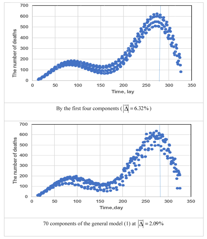
Charts of models for four and 70th components are shown in Figure 9. The vertical line separates the base and the forecast horizon.
Initially, according to the first four fluctuations from Table 2 (the model parameters were taken with 11 significant digits) with a correlation coefficient of 0.9878 (the level of adequacy of “super-strong factor relationship” with a correlation coefficient of at least 0.95), a graph was plotted in the time interval from 07/04/2020 to 31/12/2020 for the basis of the forecast and from 01/01/2021 to 14/02/2021 for the forecast horizon. Then, in the same time interval, a graph was built for all 70 components of the general model (1).
Comparison of the graphs shows their high similarity, so it turns out that it is possible to quickly identify the number of deaths by only four components.
Then the speed died allows to predict only a month and a half.
At the same time, the daily data on deaths from Covid-19 in Russia is very accurate: “The daily summary of the federal headquarters on morbidity, discharge and mortality for the previous day. It is used for prompt management decisions to assess the load on the health care system. Only promptly confirmed cases with an unambiguous diagnosis of death from coronavirus are taken into account “(according to data from the Russian website https://стопкоронавирус.рф/information/).
The forecast of the speed of all cases until 08/31/2021
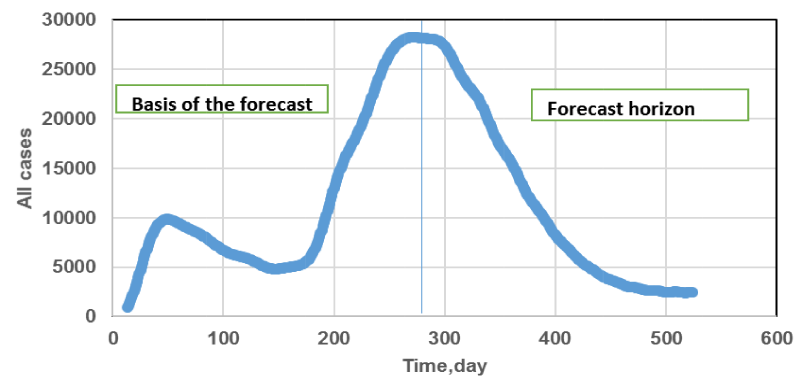
For a longer period from 01.01.2021 to 31.08.2021, that is, for eight months, the rate parameter of all cases can be predicted (Figure 10). In this case, the trigonometric formula (1) contains only seven terms, which significantly reduces the complexity of identifying asymmetric wave equations. According to Table 3, the average relative error in absolute value is only 3.22%. All cases have low stochasticity in comparison with died, which can be explained by the different vector orientation of the meaningful meaning of all four parameters taken into account.
Forecasts always depend on the measures taken by the system of government of a particular country. It may turn out that a seasonal bulge could appear in the spring of 2021. Therefore, we recommend a monthly iterative mode of identification by statistical series died and all cases with additions to the actual data for the month.
Verification of the parameters of the pandemic died and all cases
While the article was being prepared, new factual data appeared for 25 days of January 2021 (Table 5). This data turned out to be sufficient to verify the forecasts (Figure 11).
In table 5 the following conventions and expressions are adopted: , – the actual values of the speed died and all cases; , – the speed values calculated by the models died and all cases; – absolute error, person / day, and died for speed ; – relative error, for example, for speed died .
To the smallest relative error of 1.94%, the speed died before 15.01, the actual values are less than the calculated ones, and after 01/15/2021, and on the contrary, the actual values are higher than the calculated values. As a result, the 70-component model gives an outstripping decline in the number of deaths: Covid-19 in Russia is strongly resisting. Due to the permissible interval of 30%, it is impossible to predict the number of deaths beyond January 25, 2021. Then the periodicity of iterative modeling (with a shift in the beginning of the series from 03/05/2020, when in Russia all the velocity parameters did not begin to give sharp bursts) is three weeks.
For the speed of all cases, the picture is better, since the actual values decrease faster than the calculated ones. To reduce the relative modeling error, it is also recommended to carry out repeated identifications (1) every three weeks.
For four parameters of the daily dynamics of the Covid-19 pandemic in the Russian Federation, polynomial trigonometric equations were identified, including from eight (for the parameter all cases) to 70 (for the parameter died) components. It has been proven that the dynamics of a pandemic can be decomposed into individual asymmetric wavelets, which are quanta of behavior.
The identification method based on statistical daily data on four indicators of Covid-19 speed dynamics revealed quanta of pandemic behavior and responses from the healthcare system in the Russian Federation from March 25 to December 31, 2020.
The general equation (1) of an asymmetric wavelet is presented in the form of a solitary wave equation. It is shown that the speed is infected, cured, died and “all cases = infected + cured + died” in Russia got two superimposed bulges. At the same time, the large bulge will continue until the end of August 2021 for the parameter all cases. Based on the computational capabilities of the CurveExpert-1.40 software environment, a joint identification of 4-5 components was carried out with a general correlation coefficient above 0.86 for infected and more than 0.99 for all cases.
It has been proven that the spread of the virus has the form of a set of finite-dimensional wavelets with variable amplitudes and, as a rule, with a decreasing oscillation period. This is how the dynamics of the pandemic differs from the behavior of natural and natural-anthropogenic objects, which have many and infinite-dimensional wavelets with an amplitude in the form of Laplace’s law (in mathematics), Mandelbrot (in physics), Zipf-Pearl (in biology) Pareto (in econometrics).
By modeling the standard deviation by the ordinal number of the wavelet, it has been proved that the parameters of the Covid-19 pandemic also have fractal distributions. Due to finite-dimensional wavelets, the dynamics of a pandemic depends on the behavior of each country’s epidemiological system. The Russian medical system has proved to be at the proper height to counter the speed of the pandemic since April 7, 2020.
According to the computational capabilities of CurveExpert-1.40, it was found that the parameter of all cases receives the greatest adequacy with a correlation coefficient of 0.9971, in the second place with a correlation coefficient of 0.9878 is the speed died, in the third place - the speed is cured and in the fourth place - the speed is infected. Of greatest interest is the speed died.
For the velocity parameter, the first term of the trend (main bulge) has died and does not reach its maximum. And the second component of the trend reached a maximum of 164 deaths on 06/18/2020, and it will disappear from the scene of the speed dynamics died approximately from 03/23/2021. The third component, aimed at countering mortality, at the beginning of the series on March 25, 2020, received a fluctuation period of 355 days. By the date of December 31, 2020, the fluctuation period became equal to 278 days. Then, the oscillatory adaptation of physicians in Russia to the fight against mortality from Covid-19 increased only 1.28 times. More often, with constant half-periods of 3.5 and 16.1 days, fluctuations of the dead occurred. In this case, the 70th term gives a constant oscillation period, even 1.88 days.
The average relative simulation error in modulus is equal for the speed of the parameters: 1) died - 2.09; all cases - 3.22; cured - 17.17 and infected 29.91%. In this case, the range of error values among 269 values varies in the following intervals: 1) died from -18.93 to 11.95%; all cases from -31.37 to 20.20%; cured from -248.8 to 396.0%; infected from -1934.0 to 779.7%. According to the distributions of the relative error at intervals of 1%, the following rating was obtained: 1) the correlation coefficient of 0.9807 for the rate of the deceased; 2) at 0.9768 for the speed of all cases; 3) 0.8640 for the cured speed parameter; 4) 0.8174 for the speed of the infected.
The value of the standard deviation is taken as an indicator of the fractal distribution of quanta of behavior. In nature, apparently, there is no such ideal multiplicity of 2, as in Mandelbrot. As a rule, all relationships between fractal levels are non-multiple. The linear model gives the standard deviation of speeds, person/day: infected 3572.76; cured 4962.32; died 94.827 and all cases 5002.48.
Then the coefficient of total fractality will be equal to the ratio of the standard deviation of the linear model to the standard deviation of the last component, that is, to the border of quantum uncertainty. This general coefficient of fractality will be equal: for the parameter infected 3572.76 / 310.97 = 11.5; cured 5.8; died 24.3 and all cases 9.6.
Due to the high range of the relative error, the rates of cured and infected were excluded from the forecast. The range of error values among 269 values changes: 1) died from -18.93 to 11.95%; all cases from -31.37 to 20.20%.
The forecast for the rate of deaths was carried out until 02/14/2021, that is, for 44 days from 01/01/2021. The right border of the forecast horizon was adopted due to the fact that from 15.02.2021 there are negative values that are physically inadmissible.
Conclusion
The additive model makes it possible to predict the pandemic rate of all cases for a longer period from 01.01.2021 to 31.08.2021. At the same time, the trigonometric formula (1) contains only seven terms, which significantly reduces the complexity of identification. The average relative error in absolute value is only 3.22%. The parameter of all cases has a low stochasticity in comparison with the number of deaths, which can be explained by the different vector orientation of the meaning of the four parameters taken into account. To reduce the relative modeling error for these parameters of the number of deaths and in all cases, it is recommended to re-identify the asymmetric wavelet (1) every three weeks.
- Mazurkin PM (2014) Method of identification. International Multidisciplinary Scientific GeoConference, Geology and Mining Ecology Management, SGEM 427-434.
- Mazurkin PM (2015) Invariants of the Hilbert Transform for 23-Hilbert Problem. Advances in Sciences and Humanities 1: 1-12. Link: https://bit.ly/3zFDhyE
- Mazurkin PM (2015) Wavelet Analysis Statistical Data. Advances in Sciences and Humanities 1: 30-44. Link: https://bit.ly/3eWfaU7
- How epidemiology has shaped the COVID pandemic (Editorial 27 January 2021). Nature 589: 491-492. Link: https://go.nature.com/3xbA1cu
- Adam D (2020) Simulating the pandemic: What COVID forecasters can learn from climate models. Nature 587: 533-534. Link: https://go.nature.com/2VcsWLF
- Mazurkin PM, Kudryashova AI (2019) Quantum meteorology. International Multidisciplinary Scientific GeoConference Surveying Geology and Mining Ecology Management SGEM 19: 619-627.
- Adam D (2020) Special report: The simulations driving the world’s response to COVID-19. Nature 580: 316-318. Link: https://bit.ly/2UVCgDD
- Salek A, Islam S (2020) Dynamics of Covid-19 Transmission Using Mathematical Model. J Math Stat Res 2: 129. Link: https://bit.ly/372Z7jc
- Sanwal SM, Chanjiv S, Avinash V (2020) COVID-19: present and future 2.
- Amona EB, Oduro FT (2019) Modeling Ponzi scheme Propagation Dynamics: An pidemiological Approach. J Math Stat Res 1: 101. Link: https://bit.ly/2Vct51F
- Sett K (2020) On Certain Trigonometrical Sums. J Math Stat Res 2: 134.
- Mazurkin PM (2019) Wavelet analysis of annual dynamics of maximum temperature from 1878 to 2017 and forecast data Hadley center Central England temperature (Hadcet). International Journal of Current Research 11: 7315-7324. Link: https://bit.ly/2VgJKRp
Article Alerts
Subscribe to our articles alerts and stay tuned.
 This work is licensed under a Creative Commons Attribution 4.0 International License.
 Help ?

PTZ: We're glad you're here. Please click "create a new query" if you are a new visitor to our website and need further information from us.
If you are already a member of our network and need to keep track of any developments regarding a question you have already submitted, click "take me to my Query."


 Save to Mendeley