Changchun SLR data analysis using different techniques

The aim of the present study is to investigate three different techniques for fitting the SLR data observed from the Changchun observatory in China which is characterized by its huge amount of data points and to examine which of the three techniques is more proper for fitting such kind of data. The first technique is the interpolation using the Chebyshev polynomial for fitting the total number of satellite laser ranging (SLR) data points. The second technique is the spline technique which is used for matching continuous intervals for fitting the SLR data. The third technique is the method, which is used at Changchun observatory, known as the Iterative 4th order polynomial fit. The three techniques are applied to 100 samples; 50 samples for the satellite LAGEOS I and the other 50 samples for the satellite Starlette that were observed during the first quarter of 2018. From the obtained results, it is found that the first two techniques, namely the Chebyshev polynomial and Spline techniques provide better standard deviation in comparison to the Iterative 4th order polynomial fit technique that is used at Changchun observatory, with merit to Spline technique over the Chebyshev polynomial.

Introduction

One of the major challenges when dealing with a large number of data points is to fit the data with high precision in order to obtain the best results. The data under study, in the present work, is the SLR data observed by the Changchun observatory [1,2]. This data is characterized by its huge number of data points. The task of the present study is to apply three different techniques for fitting the Changchun SLR data to investigate which of the three techniques is more proper for fitting such kind of data. The first technique is the interpolation using the Chebyshev polynomial [3] for fitting the total number of satellite laser ranging data points. The second technique is the Spline technique [Micula and Micula, 1999] [4] which is used for joining continuous intervals for fitting the satellite range data. This technique is used to overcome the accumulation of errors due to a large number of mathematical operations. The third technique is the method used at Changchun observatory, namely the Iterative 4th Order polynomial fit which is applied on the range residuals (O-C residual), instead of the range measurement itself. In earlier studies, both Chebyshev and Spline techniques were examined on SLR data observed from the Helwan SLR station [5-7]. The results obtained using these two techniques are also compared with the results obtained using the technique employed at the Helwan SLR station [8,9] which uses the least square method for fitting data [7,10]. The aim of this study is to figure out the three techniques to know the more proper for fitting the Changchun-SLR data which is characterized by its very large number of data points [1]. The obtained results approved that both techniques are much better than the least square method with a great advantage of the spline technique over the Chebyshev polynomial represented by lower polynomial degree and obtained better standard deviation. Section two presents an overview of the employed techniques. Section three applies the three techniques to the Changchun SLR data for both Starlette and LAGEOS-1 satellites. The results obtained are summarized as a conclusion in section 4.

Data fitting techniques

Approximation with chebyshev polynomials: A common and direct way of data interpolation is to use polynomials and that refers to its simplest mathematical properties [6,7,10,11]. One of the popular interpolating polynomials is the Chebyshev polynomial [12]. To use the Chebyshev polynomial, the user data should be homogeneous, correlated, and transformed to be within the interval (-1, 1) [6]. Chebyshev polynomial f(x) of degree n is defined for $-1\le x\le 1$ by $f\left(x\right)=cos\theta$ where $cos\theta =x$ . It is characterized by its rapid convergence which in turn reduces the computational time and estimates the upper bound error more accurately.

In order to reach the best fit, a prepared routine under FORTRAN is used. According to the software, a comparison has been done between each two successive resulting standard deviations in order to get the best fitting. The program starts by fitting the data using the Chebyshev polynomial of the first degree (L=1) and computes the Chebyshev coefficients, followed by the generated polynomial, and the corresponding standard deviation. The routine continues the same procedure using higher polynomial degrees and tests in sequence the difference between the resulting in consecutive standard deviation until the difference becomes smaller than (5×10-5 mm; which is the proposed value to reach the best fit) [6]. Then, the program stops. Thus, the reached polynomial and the corresponding standard deviation are expected to verify the proposed condition for obtaining the best fitting. That is, the software is more suitable to determine the degree of the polynomial, in order to attain the best fitting for more explanation about the used technique, is presented [6].

Spline technique for matching continuous progressively intervals

A special form of interpolation is spline interpolation. Instead of fitting the whole data using a single, high-degree polynomial, the spline technique allows fitting subsets of the whole data using lower-degree polynomials. Fitting a large number of data points, such as Changchun SLR data, using a high-degree polynomial may suffer from noticeable errors which may destroy the accuracy of the solution [13-15]. Thus, using the spline technique to fit this kind of data leads to avoiding the roundoff errors which arise due to the nature of approximation [4]. The spline function is constructed by joining polynomials together at the endpoints of the intervals [16-18]. Also, for the Spline technique, the Chebyshev polynomial is used to fit the subintervals using the same routine mentioned in section 2.1 [16].

Iterative fitting with 4th order polynomials

In the Changchun SLR system, the normal point data is generated with the method indicated by ILRS normal point forming algorithm [19,20]. A fourth-order polynomial curve is used to fit the O-C or prediction residual (PR) dataset, to make fit the residual (FR) dataset by subtracting the curve value from PR. The FR statistics, mean and standard deviation, are then calculated. The rejection follows, by tagging data points as rejected whose FR values are off the mean by more than 2.5 times standard deviation. The fit-and-reject operation is repeated on the remaining dataset until a given iteration limit, 10 in this case. After 10 iterations, the remaining dataset is accepted for normal point formation.

Analyzing changchun SLR data

In this section, an analysis for fitting Changchun SLR data is performed using the three different techniques, for satellites Starlette and LAGEOS-1.

Fitting SLR data for starlette satellite

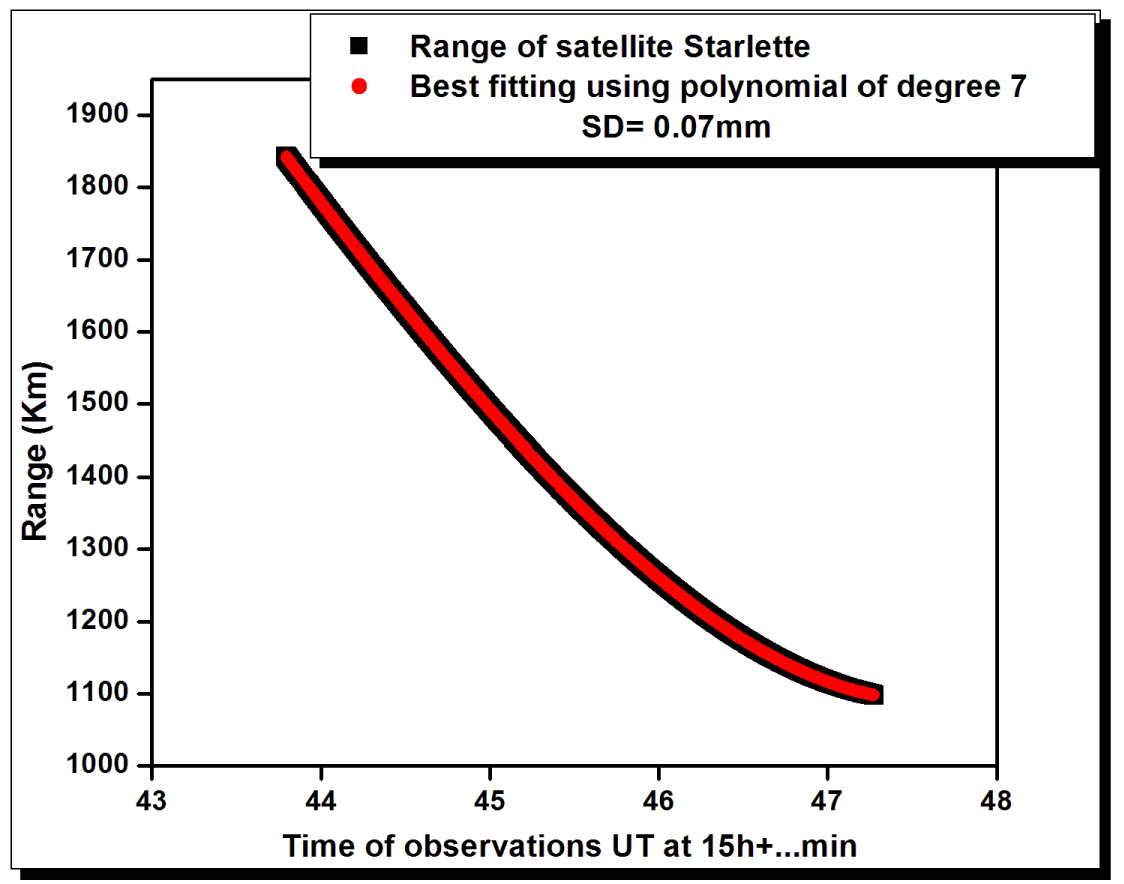
The three techniques are applied on 50 passes of satellite Starlette. As an example, figure 1 represents the whole range of satellite Starlette, which consists of 85176 data points, with its best-fitting using the Chebyshev polynomial. This pass of satellite Starlette was observed on the 4th of January 2018. The best-fitting is achieved using the polynomial of 7th degree with a corresponding standard deviation of 0.07 mm.

Figure 1: The range of satellite Starlette with its best-fitting using Chebyshev polynomial for SLR data of satellite Starlette observed at 4/1/2018.

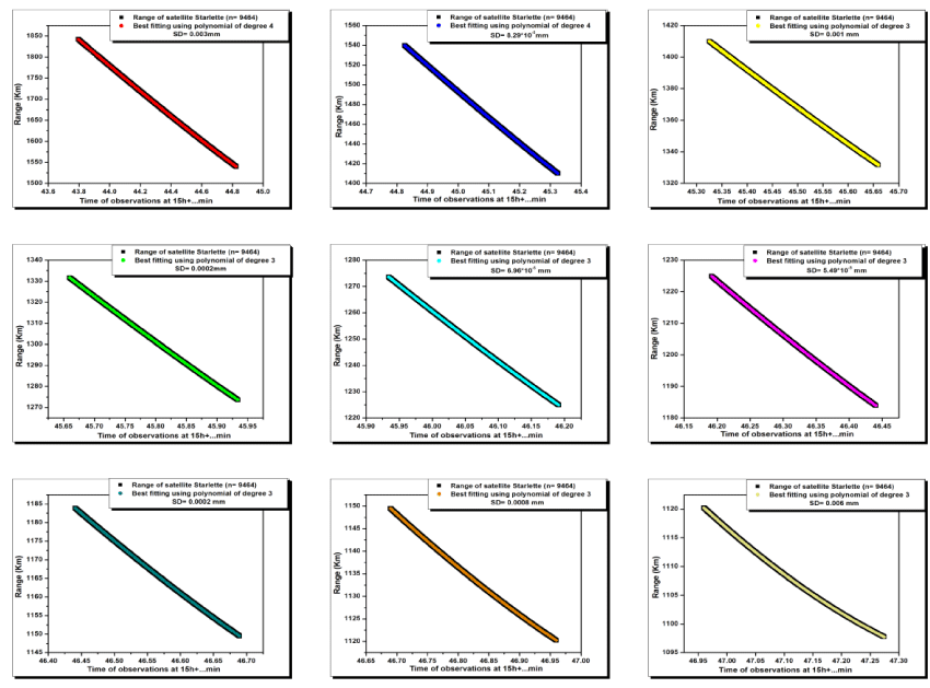
Also, the spline technique is used for fitting the SLR data of satellite Starlette which is divided into nine subintervals each of them consisting of 9464 data points.

Figure 2 shows the range of the satellite Starlette for nine subintervals with their best fit. The average polynomial degree is 3 with an average standard deviation equal to about 1.29×10-3 mm.

Figure 2: Best fitting using Spline Technique for SLR data of satellite Starlette observed at 4/1/2018.

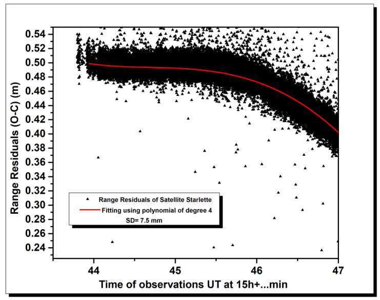
On the other hand, the Iterative fitting with 4th order polynomial, which is used at Changchun observatory is applied to the same sample. Figure 3 represents the range residual of the satellite Starlette for the total number of data points and its fitting with a polynomial of 4th degree and standard deviation of 7.5 mm.

Figure 3: The range residuals of satellite Starlette with its fitting using iterative 4th order polynomial fit observed at 4/1/2018.

Table 1 represents the polynomial degree and the corresponding standard deviation obtained by applying the three techniques on 50 passes of the satellite Starlette observed during the first quarter of 2018. The first column represents the serial number. The second column represents the total number of data points for each pass. The third and fourth columns represent the polynomial degree and its corresponding standard deviation obtained using Chebyshev polynomial for achieving the best fit. Columns five and six represent the average polynomial degree and corresponding standard deviation obtained using the Spline technique. Columns seven and eight represent the polynomial degree and the corresponding standard deviation obtained using iterative 4th order polynomial fit which is used at Changchun observatory. For comparative purposes, the average of polynomial degree and standard deviation obtained from the three techniques are calculated and represented in table 2. The results obtained show that the Spline technique allows us to use a lower polynomial degree, in comparison with using the Chebyshev polynomial for fitting the whole range data and the iterative 4th order polynomial fitting for the range residuals and still provides a better standard deviation.

Fitting SLR data for LAGEOS 1 satellite

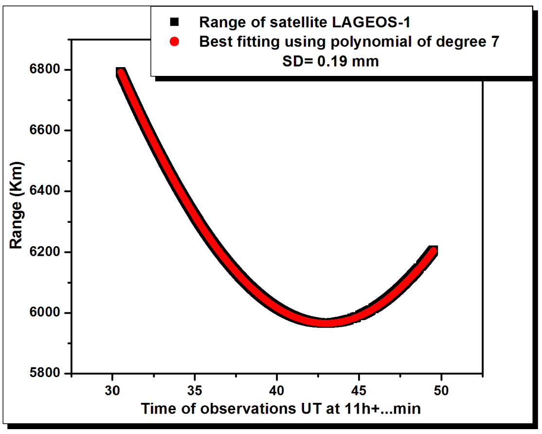
The three techniques are applied on 50 passes of satellite LAGEOS 1. As a representative example, figure 4 represents the whole range of the satellite LAGEOS-1 which consists of 80128 data points, with its best-fitting using the Chebyshev polynomial. This pass of satellite LAGEOS-1 was observed on the 12th of January 2018. The best-fitting is achieved using the polynomial of 7th degree with a corresponding standard deviation of 0.19 mm.

Figure 4: The range of satellite LAGEOS-1 with its best-fitting using Chebyshev polynomial observed at 12/1/2018.

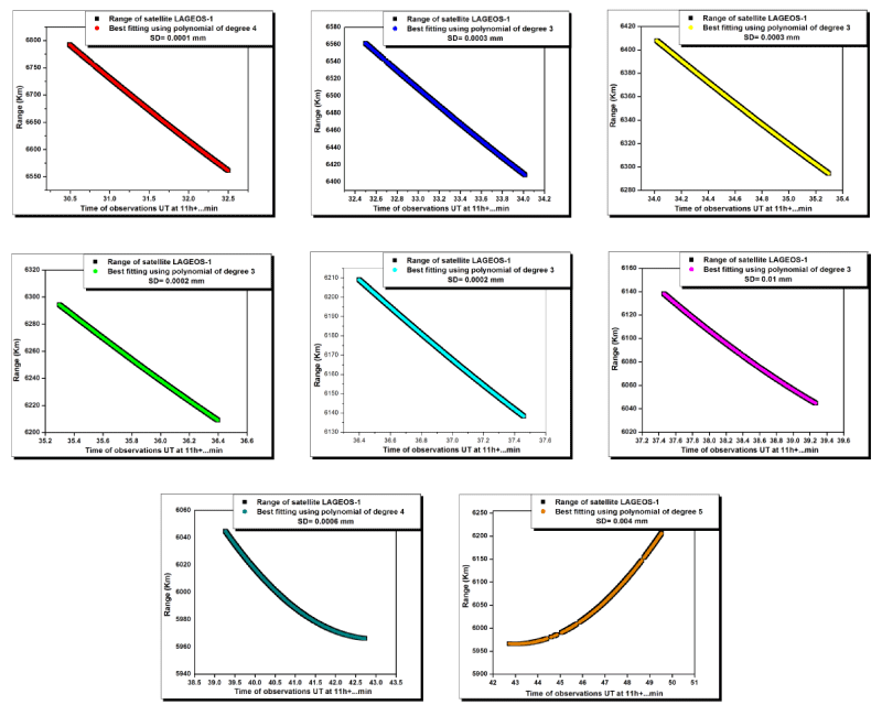
Also, the spline technique is applied. The whole data of the satellite LAGEOS-1 is divided into eight subintervals, each of which consists of 10016 data points. Figure 5 shows the range of satellite LAGEOS-1 for the eight subintervals with their best fit. The average polynomial degree is 4 with an average standard deviation equal to about 2.03×10-3mm.

Figure 5: Best fitting using Spline Technique for SLR data of satellite LAGEOS-1 observed at 12/1/2018.

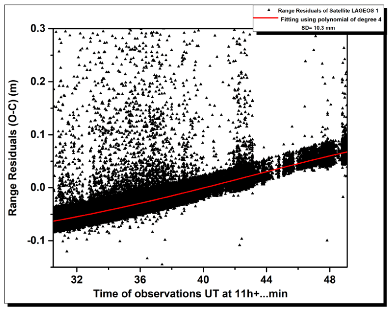
In addition, the method used at Changchun observatory; Iterative fitting with 4th order polynomials, is applied on the same pass. Figure 6 represents the range residual of the satellite Starlette for the total number of data points and its fitting with a polynomial of 4th degree and standard deviation equals 10.3 mm.

Figure 6: The range residuals of satellite Lageos-1 with its fitting using iterative 4th order polynomial fit observed at 12/1/2018.

Table 2 represents the polynomial degree and the corresponding standard deviation obtained by applying the three techniques on 50 passes of the LAGEOS-1 satellite that were observed during the first quarter of 2018. For comparative purposes, the average of polynomial degree and standard deviation for the three techniques are calculated as represented in table 2. The results obtained show that the Spline technique allows for using a lower polynomial degree for fitting a large number of data points, in comparison with the results obtained using the other two techniques and still provides a better standard deviation.

Conclusion

In a previous study, we applied the Chebyshev polynomial and the spline technique for fitting the data observed from the Helwan Satellite Laser Ranging (SLR) station [Hanna et al., 2004], and compared the results obtained; Polynomial degree and corresponding standard deviation, with the results obtained using the method employed at Helwan SLR station for fitting the data. It is found that the Spline technique has the preference over the other two techniques for fitting H-SLR data. However, Changchun-SLR data is characterized by its very large number of data points. So, the aim of this study is to figure out which of the three techniques; the Chebyshev polynomial or the spline technique, or the method used at Changchun observatory namely; Iterative 4th order polynomial fit is more proper for fitting the Changchun-SLR data. For this purpose, the three techniques are applied to 100 samples; 50 passes for satellite Starlette and 50 passes for satellite LAGEOS-1 that were observed by Changchun observatory during the first quarter of 2018. The polynomial degree and the corresponding standard deviation using the three techniques are computed and the results are summarized as a summary in Table 3. From the obtained results, it is found that both the Spline technique and Chebyshev polynomial provides better standard deviation, in comparison to the Iterative 4th order polynomial fit that is already used at the Changchun observatory. In addition, the Spline technique has the advantage of using lower polynomial degrees to reach a better standard deviation than both Chebyshev polynomial and the Iterative 4th Order polynomial Fit and still provide a better standard deviation with a difference of about one order of magnitude, on average.

For more investigation, we compared our results with that reported on the website of the International Laser Ranging Service (ILRS) for satellites Lageos1 and Starlette observed by Changchun observatory for the first quarter of 2018 https://ilrs.gsfc.nasa.gov/network/system_performance/global_report_cards/1997-2019/perf_2018q1_wLLR.html and fitted using the Iterative 4th order polynomial Fit technique. The standard deviation is 9.6 mm and 7.8 mm for the satellites LAGEOS-1 and Starlette respectively, which approves that both the Chebyshev polynomial and Spline techniques can be better choices for fitting such large amount of data points as Changchun-SLR data, with the merit of Spline technique over the Chebyshev polynomial.

1. Liang Z, Dong X, Ibrahim M, Song Q, Han X, Liu Ch, Zhang H, Zhao G. Tracking the space debris from the Changchun Observatory. Astrophys Space Sci. 2019; 364: 201.
2. Zhao Y, Fan CB, Han X, Zhao G, Zhang Z, Dong X, Zhang HT, Shi JY. Progress in Changchun SLR. Proceedings of the 16th International Workshop on Laser Ranging, Poznan, Poland. 2008. 525–530.
3. Mason JC, Handscomb DC. Chebyshev Polynomials. Chapman & Hall, New York. 2003.
4. Micula G, Micula S. Handbook of Splines. Kluwer, Dordrecht 1999.
5. Hanna YS, Ibrahim M, Samwel SW. Spline and overlap techniques for analyzing SLR data, Space Res J. 2012; 5(1): 1–9.
6. Samwel SW, Hanna YS, Ibrahim M. On applying the spline technique for fitting different kinds of data. NRIAG J Astron Astrophys. 335–345. 2004.
7. Hanna YS, Ibrahim M, Samwel SW. On using Chebyshev polynomial for fitting SLR data of artificial satellites. Applied Math Comput. 2004; 158: 655-666.
8. Ibrahim M, Hanna YS, Samwel SW, Hegazy MA. Satellite Laser Ranging in Egypt, NRIAG Journal of Astronomy and Geophysics. 2015; 4:123-129.
9. Ibrahim M. 17 years of ranging from the Helwan-SLR station, Astrophysics and Space Science Journal. 2011; 335: 379-387.
10. Samwel SW, Hanna YS, Ibrahim M, Roman AT. Overlap technique for fitting the range residuals of the SLR data. NRIAG Journal of Astronomy and Geophysics. 2015; 4: 293–297.
11. Nielsen Kaj L. Methods in Numerical Analysis. MacMillan Company, Collier MacMillan limited, New York, London.
12. Fox L, Parker IB. Chebyshev Polynomials in Numerical Analysis, Oxford University Press. 1968.
13. Angeles J. Fundamentals of Robotic Mechanical Systems, Theory, Methods, and Algorithms, fourth ed., Springer. 2014.
14. Lindfield GR, Penny JET. Numerical Methods: Using MaTLAB, third ed. Academic Press, Elsevier. 2012.
15. Gottlieb S, Jung JH. Numerical issues in the implementation of high order polynomial multi-domain penalty spectral Galerkin methods for hyperbolic conservation laws. Commun Comput Phys. 2012; 5: 600–619.
16. Hanna YS, Ibrahim M, Samwel SW. Spline and overlap techniques for analyzing SLR data. Space Res J. 2012; 5(1): 1–9.
17. Hama-Salh FK. Inhomogeneous lacunarry interpolation by splines (0,2;0,1,4) case. Asian J Math Stat. 2010; 3: 211-224.
18. Nmadu JN, Yisa ES, Mohammed US. Spline functions: Assessing their forecasting consistency with changes in the type of model and choice of joint pints. Trends Agric Econ. 2009; 2:17-27.
19. NPTAlgo. Feb 28, 2018, https://ilrs.gsfc.nasa.gov/data_and_products/data/npt/npt_algorithm.html
20. Ibrahim M, Abd El-Hameed AM, Liang Z, Han X. Analytical investigation for the satellite ranging data of Changchun-SLR station. NRIAG Journal of Astronomy and Geophysics. 2020; 9: 321-329. DOI: 10.1080/20909977.2020.1743914