Convolutional modelling of epidemics

Traditional deterministic modeling of epidemics is usually based on a linear system of differential equations in which compartment transitions are proportional to their population, implicitly assuming an exponential process for leaving a compartment as happens in radioactive decay. Nonetheless, this assumption is quite unrealistic since it permits a class transition such as the passage from illness to recovery that does not depend on the time an individual got infected. This trouble significantly affects the time evolution of epidemy computed by these models. This paper describes a new deterministic epidemic model in which transitions among different population classes are described by a convolutional law connecting the input and output fluxes of each class. The new model guarantees that class changes always take place according to a realistic timing, which is defined by the impulse response function of that transition, avoiding model output fluxes by the exponential decay typical of previous models. The model contains five population compartments and can take into consideration healthy carriers and recovered-to-susceptible transition. The paper provides a complete mathematical description of the convolutional model and presents three sets of simulations that show its performance. A comparison with predictions of the SIR model is given. Outcomes of simulation of the COVID-19 pandemic are discussed which predicts the truly observed time changes of the dynamic case-fatality rate. The new model foresees the possibility of successive epidemic waves as well as the asymptotic instauration of a quasi-stationary regime of lower infection circulation that prevents a definite stopping of the epidemy. We show the existence of a quadrature function that formally solves the system of equations of the convolutive and the SIR models and whose asymptotic limit roughly matches the epidemic basic reproduction number.

Introduction

The current COVID-19 pandemic highlights the relevance of reliable theoretical modelings able to provide correct predictions of epidemy propagation and extension. In the recent past, a great effort has been devoted to trying to give correct representation to such phenomena as infection latency before symptoms onset, the time required for healing, the role of asymptomatic individuals in epidemy propagation [1,2] and so forth. Several authors [3-8] have attempted to improve the likelihood of deterministic modelings trying to increase the number of model compartments or introducing a delay between the time of pathogen exposition and that of inclusion in the infected compartment [8-14]. Other works [15-17] have investigated the ability to predict epidemic dynamics of distributed delay models, which represent delays by introducing differential equations convolutions with some functions that model class transitions. Unfortunately, these modelings (delayed and time distributed) do not guarantee that time elapsed between exposition and illness is correctly distributed because they act on compartment populations rather than on fluxes among them. Despite expectations, these models do not control the time interval between entering and leaving a given class (compartment) and how this time lag is distributed when considering many class transitions. Moreover, the delay is usually introduced to model the incidence rate, while all other passages between different compartments only rarely are delayed. Nonetheless, also these class transitions need a realistic time distribution for the theoretical model to be able to provide realistic predictions of epidemic propagation. Evidently, this lack of likelihood can reduce the accuracy of quantitative predictions forecasted by these models when investigating epidemic evolutions. This point, which will be discussed in the following, has also been addressed in [18] although in the framework of stochastic modeling. Many authors have investigated the effects on the dynamical behavior of deterministic models when including in their equations a nonlinear incidence or recovery rate [19-23], proving the occurrence of bifurcations [24]. The nonlinear terms originated trying to include into the model the effects of systemic phenomena such as the availability of hospital beds on the recovery rate, or restrictive measures dictated by governments. The mathematical formulation of these nonlinearities is however arbitrary, and no way exists to prove the physical foundation of different models of the same phenomenon. Din et al [25,26] have proposed the application of fractional order Atanganaa–Baleanu Caputo derivative to the theoretical modeling of the Hepatitis B epidemic, also differentiating acute infected from chronically infected individuals. An emerging approach is the application of data assimilation techniques to the standard or a modified version of the SIR model [27]. This option leads to a modified Kalman filter, which would be specifically suited to solve the problem of parameter estimation stemming from epidemic data.

In this paper, we outline a new type of deterministic epidemic modeling that include five population compartments and introduces the concept of fluxes among them. Classes are considered time-invariant linear systems that connect the input to output fluxes, making it possible to account for the time evolution of each population class. The model guarantees a parametric temporal distribution of infection evolution that is dictated by the impulse response function associated with each class transition. Due to its mathematical structure, the new model prevents impossible phenomena (class transitions) such as some population fraction that persists into the infected class for a too short (e.g.: null), or too long (e.g.: years), time interval. The model can allow restored people to come back into the susceptible class, giving rise to successive epidemic peaks, and predicts the existence of “evanescent” epidemic waves circulating for a long time even for basic reproduction numbers less than a unit. Due to its mathematical structure, the model holds thirteen free parameters that can fit its behavior to different kinds of diseases.

The paper shows the outcomes of simulations executed to assess the performance of the new model in comparison with the SIR, and for the current COVID-19 pandemic.

The remainder of this paper is organized as follows. In Sect. 2.0 a self-contained description of the mathematical structure of the model is given, highlighting the main mathematical differences with previous epidemic modelings (e.g.: the SIR). Sect. 3.0 reports the software implementation of the model that has been adopted to perform simulations of epidemics shown in Sect. 4.0. Here three sets of simulations are shown that demonstrate the model's capability to foresee successive epidemic waves, its ability to account for some phenomena typical of the COVID-19 pandemic and its asymptotic behavior. Sect. 5.0 resumes the principal findings of this work.

Material and methods

The convolutional model of epidemics

• The new model assumes that the whole population can be divided into five classes, as specified below.
•  The susceptible class s(t) contains those individuals who can be infected.
• Exposed individuals e(t) got in contact with the pathogen but do not have developed the related illness yet.
• Infected/sick class i(t) is constituted by persons who fell ill.
• Restored r(t); those people who recovered from infection of, or exposition to, the pathogen agent.
• Deceased class d(t). Individuals who died due to the infectious agent.

We assume the above functions of time are relative abundances (frequencies) of the corresponding class normalized to the whole population, with unitary sum s(t)+ e(t)+ i(t)+ r(t)+ d(t) = 1. Class transitions happen according to the scheme of Figure 1.

Figure 1: Layout of the new convolutional model. The symbols Φ… (t) represents the fluxes among the various population categories (fraction of people that in the time unity flows from one category to another).

It is worth noting that a part of the exposed persons can turn into the restored class as being healthy carriers or quasi-asymptomatic, while a fraction of restored people can become newly susceptible.

Fluxes among classes in Figure 1 are input and output derivatives of the related class abundances, as exemplified in the relationship below for the flux ${\text{Φ}}_s\left(t\right)$ between the susceptible and exposed:

${\Phi }_s\left(t\right)=-\frac{d{s}_{Out}\left(t\right)}{dt}=\frac{d{e}_{Inp}\left(t\right)}{dt}\ge 0\text{ (1)}$

We assume that fluxes and input derivatives always are non-negative, while output derivatives are non-positive. With this convention, the algebraic sum of input and output derivatives equates to the total time derivative that can be written as a function of fluxes.

$\{\begin{array}{c}\frac{ds\left(t\right)}{dt}=-{\text{Φ}}_s\left(t\right)+{\text{Φ}}_r\left(t\right)\\ \frac{de\left(t\right)}{dt}={\text{Φ}}_s\left(t\right)-{\text{Φ}}_{ei}\left(t\right)-{\text{Φ}}_{er}\left(t\right)\\ \frac{di\left(t\right)}{dt}={\text{Φ}}_{ei}\left(t\right)-{\text{Φ}}_{ir}\left(t\right)-{\text{Φ}}_{id}\left(t\right)\\ \frac{dr\left(t\right)}{dt}={\text{Φ}}_{er}\left(t\right)+{\text{Φ}}_{ir}\left(t\right)-{\text{Φ}}_r\left(t\right)\\ \frac{dd\left(t\right)}{dt}={\text{Φ}}_{id}\left(t\right)\end{array}$

The system of equations (2) needs to be completed by additional equations that specify the rules for computing the six fluxes.

All fluxes, except ${\text{Φ}}_s\left(t\right)$ , are calculated according to a convolutional model that links the input signal (flux) of a class with its output, adding delay and spreading which are regulated by the Impulse Response Functions (IRFs) characteristic of each class transition. These IRFs are representative of specific biophysical phenomena, such as the incubation period of the disease (for e(t) to i(t) transition) or the healing time i(t) (to r(t)). IRFs are indicated in Figure 1 near the exit fluxes of each class.

Let us consider the Input/Output (I/O) relationship for a generic class with an input flux ${\text{Φ}}_{Inp}\left(t\right)$ and an exit flux ${\text{Φ}}_{Out}\left(t\right)$ . The relative population abundance ${\text{Φ}}_{Inp}\left(\tau \right)d\tau$ entering the class between τ and τ + dτ is subsequently transferred into the output flux at time t according to the IRF $h\left(t-\tau \right)$ :

$d{\text{Φ}}_{Out}\left(t\right)={\text{Φ}}_{Inp}\left(\tau \right)d\tau h\left(t-\tau \right)\text{ (3)}$

This equation implies that class transition is stationary (aka Time-Invariant, TI): delaying the input flux results in a delayed version of the output flux without affecting its profile. Assuming the epidemy broke out at time t = 0 (all fluxes are zero for negative times), we find the total output flux at the time t by integrating the input contributions over all the instants τ preceding t:

${\text{Φ}}_{Out}\left(t\right)={{\displaystyle \int }}_0^t{\text{Φ}}_{Inp}\left(\tau \right)h\left(t-\tau \right)d\tau ={{\displaystyle \int }}_{-\infty }^{+\infty }{\text{Φ}}_{Inp}\left(\tau \right)h\left(t-\tau \right)d\tau \text{ (4)}$

The right-hand side of Eq. (4) is the convolution between the input flux and the IRF for the considered class transition, meaning that class transitions behave like a TI Linear System (LS). The causality of this LS is guaranteed since admitted IRFs are null for negative values of their argument (input time τ in the future of the output time t). This feature allows us to arbitrarily extend the upper bound of the integral on the right-hand-side of Eq. (4). Conservation of the relative number of individuals throughout the class transition is guaranteed by the unitary area of function h(t). These conditions are recapped by the following equations.

$\{\begin{array}{c}h\left(t\right)=0 \forall t<0\\ {\int }_0^{+\infty }h\left(\tau \right)d\tau =1\end{array}\text{ (5)}$

We propose gaussian IRFs for our model, bell-shaped functions that are frequently adopted to fit epidemic data [28] and that avoid unrealistic wings for large t. However, the IRS's profile may be characteristic of the modeled disease and should be adapted accordingly. A typical instance of gaussian IRF is detailed in Eq. (6) where T is the average delay of class transition taking place and σ it's spreading.

$h\left(t\right)=\frac{A}{\sqrt[2]{2\pi {\sigma }^2}}\text{exp}\left[-\frac{{\left(t-T\right)}^2}{2{\sigma }^2}\right]\text{ (6)}$

Whenever the flux ${\text{Φ}}_s\left(t\right)$ is known, the iterative application of Eq. (4) to each class of Figure 1 leads to the determination of all other fluxes.

To ascertain the flux ${\text{Φ}}_s\left(t\right)$ , it is necessary to find the probability dP0 for a susceptible to come in contact with the pathogen in a given time interval dt. dP0 is given by the average frequency of encounters f0 between two individuals of that population multiplied by the conditional probability that one belongs to the susceptible class and the other to the exposed or infected classes. We assume that exposed and infected individuals can both transmit the infection, a characteristic that seems important for such diseases as COVID-19. This probability is outlined by the equation below:

$d{P}_0=f_{0}2\frac{e\left(t\right)s\left(t\right)}{{\left[1-d\left(t\right)\right]}^2}dt+f_{0}2\frac{i\left(t\right)s\left(t\right)}{{\left[1-d\left(t\right)\right]}^2}dt\text{ (7)}$

A casual encounter between a susceptible and an individual of class i(t) or e(t) can happen in two distinct orders generating factor 2 on the right-hand side of Eq. (7), and the subsequent Eqs. (8,9). If the two individuals are indicated as A and B, the encounter between a susceptible and an infected takes place either as $A\in i\left(t\right),B\in s\left(t\right)$ , or as $B\in i\left(t\right),A\in s\left(t\right)$ , both with probability $\frac{i\left(t\right)s\left(t\right)}{{\left[1-d\left(t\right)\right]}^2}$ . The probability that a randomly chosen individual belongs to the infected compartment is $\frac{i\left(t\right)}{1-d\left(t\right)}$ , and the correction factor $\left[1-d\left(t\right)\right]$ is the total living population and expresses the condition that dead individuals cannot participate in encounters. Previous models [3,29] neglect this correction, underestimating the conditional probability of casual encounters. Only a fraction of these contacts, called transmissibility, can truly transmit the pathogen, and this factor should be lesser for exposed than infected people. Let b indicate the transmissibility for infected individuals, and ε . b, with $\epsilon \le 1$ , be the transmissibility of exposed ones. Multiplying the two addenda of dP0 by the respective transmissibility, we obtain the people's amount ${\text{Φ}}_s\left(t\right)dt$ leaving the susceptible class within the time interval dt:

${\text{Φ}}_s\left(t\right)dt=2\epsilon .b\cdot f_0\frac{e\left(t\right)s\left(t\right)}{{\left[1-d\left(t\right)\right]}^2}dt+2b\cdot f_0\frac{i\left(t\right)s\left(t\right)}{{\left[1-d\left(t\right)\right]}^2}dt\text{ (8)}$

This relationship can be conveniently condensed as shown in Eq. (9):

$\begin{array}{c}k=b{f}_0\\ {\Phi }_s\left(t\right)=2k\frac{\left[\epsilon \cdot e\left(t\right)+i\left(t\right)\right]s\left(t\right)}{{\left[1-d\left(t\right)\right]}^2}\end{array}\text{ (9)}$

Using this outcome, it is possible to write the equations that govern the time evolution of I/O fluxes.

$\{\begin{array}{l}{\Phi }_s\left(t\right)=2k\frac{\left[\epsilon e\left(t\right)+i\left(t\right)\right]s\left(t\right)}{{\left[1-d\left(t\right)\right]}^2}\\ {\Phi }_{ei}\left(t\right)=\left(1-\alpha \right)\cdot \underset{}{\overset{}{{\displaystyle {\int }_0^{+t}}}}{\Phi }_s\left(\tau \right)h_e\left(t-\tau \right)d\tau \\ {\Phi }_{er}\left(t\right)=\alpha \cdot \underset{}{\overset{}{{\displaystyle {\int }_0^{+t}}}}{\Phi }_s\left(\tau \right)h_e\left(t-\tau \right)d\tau \\ {\Phi }_{ir}\left(t\right)=\beta \cdot \underset{}{\overset{}{{\displaystyle {\int }_0^{+t}}}}{\Phi }_{ei}\left(\tau \right)h_{ir}\left(t-\tau \right)d\tau \\ {\Phi }_{id}\left(t\right)=\left(1-\beta \right)\cdot \underset{}{\overset{}{{\displaystyle {\int }_0^{+t}}}}{\Phi }_{ei}\left(\tau \right)h_{id}\left(t-\tau \right)d\tau \\ {\Phi }_r\left(t\right)=\gamma \cdot \underset{}{\overset{}{{\displaystyle {\int }_0^{+t}}}}\left[{\Phi }_{er}\left(t\right)+{\Phi }_{ir}\left(t\right)\right]h_r\left(t-\tau \right)d\tau \end{array}\text{ (10)}$

$\{\begin{array}{c}{h}_e\left(t\right)=\frac{A_{e}u\left(t\right)}{\sqrt[2]{2\pi {\sigma }_e^2}}exp\left[-\frac{{\left(t-T_e\right)}^2}{2{\sigma }_e^2}\right]\\ h_{ir}\left(t\right)=\frac{A_{ir}u\left(t\right)}{\sqrt[2]{2\pi {\sigma }_{ir}^2}}exp\left[-\frac{{\left(t-T_{ir}\right)}^2}{2{\sigma }_{ir}^2}\right]\\ h_{id}\left(t\right)=\frac{A_{id}u\left(t\right)}{\sqrt[2]{2\pi {\sigma }_{id}^2}}exp\left[-\frac{{\left(t-T_{id}\right)}^2}{2{\sigma }_{id}^2}\right]\\ h_r\left(t\right)=\frac{A_{r}u\left(t\right)}{\sqrt[2]{2\pi {\sigma }_r^2}}exp\left[-\frac{{\left(t-T_r\right)}^2}{2{\sigma }_r^2}\right]\end{array}\text{ (11)}$

Eqs. (2,10-11) form the new convolutional model described in this work. The four parameters A_e, A_ir, A_id, and A_r are area normalization constants of the related IRFs and are implicit functions of the delay and dispersion. u(t) is the Heaviside step function that makes IRFs null for negative values of their argument, α [1-α] is the fraction of exposed people who recover without developing illness [fall sick], and β [1-β] is the fraction of sick individuals who recover [die].

Remarkably, the output fluxes in the epidemic model discussed in this work are not represented by a decay process as happens in almost all deterministic epidemic modelings [3, 4, 15, 27, 29, 30]. It should be noted that the exponential decay is an improbable assumption for epidemic models because the output flux is proportional to the abundance of the considered class irrespective of when people entered it. Due to this essential feature, the convolutional model avoids impossible or implausible events such as the recovery or death of infected people immediately after their infection. In different wording, the model herein discussed can provide a realistic timing for the passage of population fractions among existing model compartments.

Let us note that while each class population is the probability that a randomly selected individual belongs to that class, the IRFs h(t-τ) are proportional to conditional probability functions; i.e.: the probability that an individual leaves the considered class at time t provided that he entered that class at time τ ≤ t. In different wording, IRFs behave like “time propagators” for fluxes among classes and, indirectly, for class probabilities(s(t), e(t), i(t), r(t), and d(t)).

Table 1 details the free parameters of Eqs. (10,11) necessary to fit the model to the epidemy of interest. The possibility that recovered persons turn back into the susceptible class can be precluded by taking γ = 0.

The two output fluxes of the class i(t) are regulated by different IRFs, h_ir (t) toward the restored class and h_id (t) toward the deceased class. This means that this model can provide different timing of evolution for the fraction of infected people who die with respect to those who survive the disease.

The asymptotic behavior

Due to the IRFs‘ normalization, the overall death rate of the new model equates (1-α).(1-β). Whenever γ = 0, the asymptotic limit of susceptible and death classes ( $s_{\infty }=\underset{t\to +\infty }{\lim }s\left(t\right)$ and) $d_{\infty }=\underset{t\to +\infty }{\lim }d\left(t\right)$ are linked together with the death rate by the simple relationship shown below:

$d_{\infty }=\left(1-s_{\infty }\right)\cdot \left(1-\alpha \right)\cdot \left(1-\beta \right)\text{ (12)}$

The convolutional model admits a quasi-stationary solution in which i(t) and e(t) are almost constant, with vanishing derivatives. Imposing this condition into Eqs. (2) leads to the equations below.

$\{\begin{array}{c}\frac{de\left(t\right)}{dt}=0\to {\text{Φ}}_s\left(t\right)={\text{Φ}}_{ei}\left(t\right)+{\text{Φ}}_{er}\left(t\right)\\ \frac{di\left(t\right)}{dt}=0\to {\text{Φ}}_{ei}\left(t\right)={\text{Φ}}_{ir}\left(t\right)+{\text{Φ}}_{id}\left(t\right)\end{array}\text{ (13)}$

Substituting the second of these relationships into the first, we obtain:

${\text{Φ}}_s\left(t\right)={\text{Φ}}_{ir}\left(t\right)+{\text{Φ}}_{id}\left(t\right)+{\text{Φ}}_{er}\left(t\right)\text{ (14)}$

Eq. (14) proves that in this regime the decrease of susceptibles is continuously absorbed by the restored and deceased classes, apart from the ${\text{Φ}}_r\left(t\right)$ flux transporting recovered persons back into the susceptible class. Simulations performed with our model show this asymptotic behavior for large t frequently.

Basic reproduction number

The estimation of the basic reproduction number [31] of the convolutive model is made complex by the circumstance that two classes, e(t) and i(t), can transmit the infection, giving rise to three outflows having different time constants. Using the same flux weighting shown in Eqs. (10-11) we write:

$R_0\cong 2\epsilon k\alpha \cdot T_e+2k\left(1-\alpha \right)\cdot \left[\epsilon T_e+\beta T_{ir}+\left(1-\beta \right)T_{id}\right]\text{ (15)}$

• The standard deviation of each IRF is far below the related delay; e. g.: ${\sigma }_e\ll T_e$ . Whenever the standard deviation is comparable to (or greater than) the delay, the integration domain only includes a small slice of the left flank of the IRF, hence the integral is dominated by contributions originating on the right flank of the IRF. In this case, exposed and infected individuals propagate the disease for an average time greater than the delay.
• γ = 0 and the overall death rate is small, thus no correction for the division by the ${\left[1-d\left(t\right)\right]}^2$ the factor is necessary.
• The epidemy is in its starting phase $s\left(t\right)~1$ .

A formal solution to epidemic equations

Whenever γ = 0 the fundamental equation of the convolutional model reduces to:

$\frac{1}{s\left(t\right)}\frac{ds\left(t\right)}{dt}=-2k\frac{\left[\epsilon e\left(t\right)+i\left(t\right)\right]}{{\left[1-d\left(t\right)\right]}^2}\text{ (16)}$

Introducing a new function of time p(t) defined as the primitive of $2k\frac{\left[\epsilon e\left(t\right)+i\left(t\right)\right]}{{\left[1-d\left(t\right)\right]}^2}$ , and performing simple mathematical manipulations a formal solution of the model is obtained:

$\{\begin{array}{c}p\left(t\right)=2k{\int }_o^t\frac{\left[\epsilon e\left(\tau \right)+i\left(\tau \right)\right]}{{\left[1-d\left(\tau \right)\right]}^2}d\tau \\ s\left(t\right)=s\left(0\right)e^{-p\left(t\right)}\end{array}\text{ (17)}$

Expressing the other classes as a function of p(t) is rather complex and is neglected. Let us note that a similar solution can be obtained for almost any deterministic epidemic model, as for the SIR (Eqs. (18)) whose complete formal solution is shown by Eqs. (19):

$\{\begin{array}{c}{s}^{\text{'}}\left(t\right)=-k\cdot i\left(t\right)s\left(t\right)\\ i^{\text{'}}\left(t\right)=k\cdot i\left(t\right)s\left(t\right)-\frac{1}{T_{SIR}}i\left(t\right)\\ r^{\text{'}}\left(t\right)=\frac{1}{T_{SIR}}i\left(t\right)\end{array}\text{ (18)}$

$\{\begin{array}{c}p\left(t\right)=k{\int }_o^{t}i\left(\tau \right)d\tau \\ s\left(t\right)=s\left(0\right)e^{-p\left(t\right)}\\ i\left(t\right)=1-s\left(0\right)e^{-p\left(t\right)}-\frac{1}{T_{SIR}}p\left(t\right)\\ r\left(t\right)=\frac{1}{T_{SIR}}p\left(t\right)\end{array}\text{ (19)}$

Eqs. (17,19) is the quadrature of the related epidemic model but since the function p(t) remains unknown they do not permit us to deduce the epidemy evolution, thus they are formal solutions to the related problems. Nonetheless, they can be useful to interpret the outcome of simulations discussed in the next Sections.

Model implementation

Model implementation has been made by developing a custom software code utilizing the C/C++ programming language. The systems of coupled integrodifferential equations given by Eqs. (2,10,11) have been solved by adopting Euler’s method with a discrete time step ∆t far below the least standard deviation among the four IRFs of Eqs. (11). Discrete time evolution equations are recapped below, where the symbol * represents convolution, while the apex stands for time derivative.

$t_n=n\cdot \Delta t\text{ (20)}$

$\{\begin{array}{c}s\left[n\right]=s\left[n-1\right]+s\text{'}\left[n-1\right]\cdot \Delta t\\ e\left[n\right]=e\left[n-1\right]+e\text{'}\left[n-1\right]\cdot \Delta t\\ i\left[n\right]=i\left[n-1\right]+i\text{'}\left[n-1\right]\cdot \Delta t\\ r\left[n\right]=r\left[n-1\right]+r\text{'}\left[n-1\right]\cdot \Delta t\\ d\left[n\right]=d\left[n-1\right]+d\text{'}\left[n-1\right]\cdot \Delta t\end{array}\text{ (21)}$

$\{\begin{array}{l}{\Phi }_s\left[n\right]=2k\frac{\left[\epsilon \cdot e\left[n\right]+i\left[n\right]\right]s\left[n\right]}{{\left[1-d\left[n\right]\right]}^2}\\ {\Phi }_{ei}\left[n\right]=\left(1-\alpha \right)\cdot {\Phi }_s\left[n\right]*h_e\left[n\right]\\ {\Phi }_{er}\left[n\right]=\alpha \cdot {\Phi }_s\left[n\right]*h_e\left[n\right]\\ {\Phi }_{ir}\left[n\right]=\beta \cdot {\Phi }_{ei}\left[n\right]*h_{ir}\left[n\right]\\ {\Phi }_{id}\left[n\right]=\left(1-\beta \right)\cdot {\Phi }_{ei}\left[n\right]*h_{id}\left[n\right]\\ {\Phi }_r\left[n\right]=\gamma \cdot \left\{{\Phi }_{er}\left[n\right]+{\Phi }_{ir}\left[n\right]\right\}*h_r\left[n\right]\end{array}\text{ (22)}$

$\{\begin{array}{c}s\text{'}\left[n\right]=-{\text{Φ}}_s\left[n\right]+{\text{Φ}}_r\left[n\right]\\ e\text{'}\left[n\right]={\text{Φ}}_s\left[n\right]-{\text{Φ}}_{ei}\left[n\right]-{\text{Φ}}_{er}\left[n\right]\\ i\text{'}\left[n\right]={\text{Φ}}_{ei}\left[n\right]-{\text{Φ}}_{ir}\left[n\right]-{\text{Φ}}_{id}\left[n\right]\\ r\text{'}\left[n\right]={\text{Φ}}_{er}\left[n\right]+{\text{Φ}}_{ir}\left[n\right]-{\text{Φ}}_r\left[n\right]\\ d\text{'}\left[n\right]={\text{Φ}}_{id}\left[n\right]\end{array}\text{ (23)}$

Results and discussion

Simulations aim at demonstrating specific features of the convolutional model, comparing its performance to those achieved by the SIR model [29], and investigating some aspects of the COVID-19 pandemic. Unfortunately, available data for this epidemy show significant differences among different countries concerning sampling methods and classification of deaths, hence comparison between theoretical predictions and real data will be made at a qualitative level. All simulations have been computed starting the infection at t = 0 with a $i\left(t=0\right)={10}^{-6}$ exposed persons. The SIR model has also been solved utilizing Euler’s approach.

Simulation #1

In this simulation, we have investigated an important issue of epidemics, i.e., the formation of oscillatory epidemic propagation modes that have been reported during the current COVID-19 epidemic frequently [32]. We have selected the model-free parameters shown in Table 2 where time constants (T,σ) are expressed in days. The value γ = 0.8 has been chosen to investigate the model's ability to foresee successive epidemic waves that are summarized in Figure 2.

Let us note that the new model can reproduce oscillating temporal patterns of epidemics, which are forced by the high value imposed on the γ parameter. However, simulated oscillatory patterns always are damped, hence for a large time, the model reproduces the quasi-stationary regime dictated by Eqs. (13-14) notwithstanding the large γ value. The period of such oscillations seems to slightly increase with increasing time.

Simulation #2

Simulation #2 aims at elucidating the principal difference between the standard SIR and the new epidemic convolutional model discussed in this work. The parameters of this simulation roughly represent the COVID-19 pandemic. The maximum incubation period is believed to not exceed 14 days [33-37] with an average between 5.1 days [35,36] and 8 days [34], so we have chosen $T_e=8$ days and ${\sigma }_e=4$ days. The fatality rate has been estimated between 2.2% [35], 3.8% [33], and 5.6% [37] (4% in our simulation), while the time between symptom onset and death ranged from about 2 weeks to 8 weeks in [33], was estimated to be 8 days in [38] and 11 days in [39] $T_{id}=11$ (days and ${\sigma }_{id}=5$ days in this simulation). A recovery time of 2 weeks for patients with mild symptoms (3-6 weeks for patients in critical conditions) has been reported in [33], which we have condensed with $T_{ir}=18$ days, ${\sigma }_{ir}=7$ days. The remaining parameters of this simulation were: γ = 0 ( $T_r$ and ${\sigma }_r$ are ineffectual), $T_{SIR}=12,415$ days, $R_0=R_0\left(SIR\right)\cong 2.483$ (2.2 in [35], between 2.8 and 3.9 in [36]).

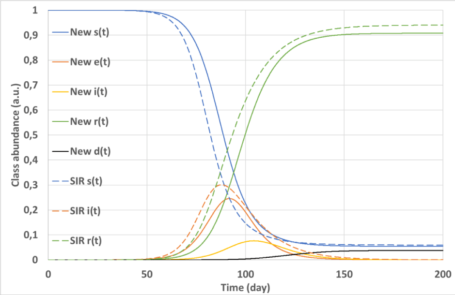
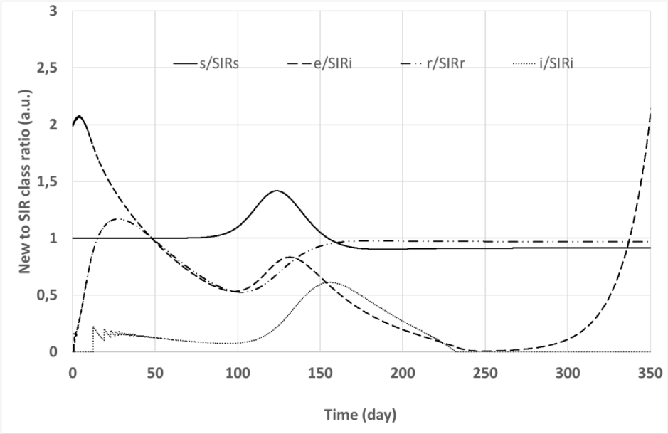
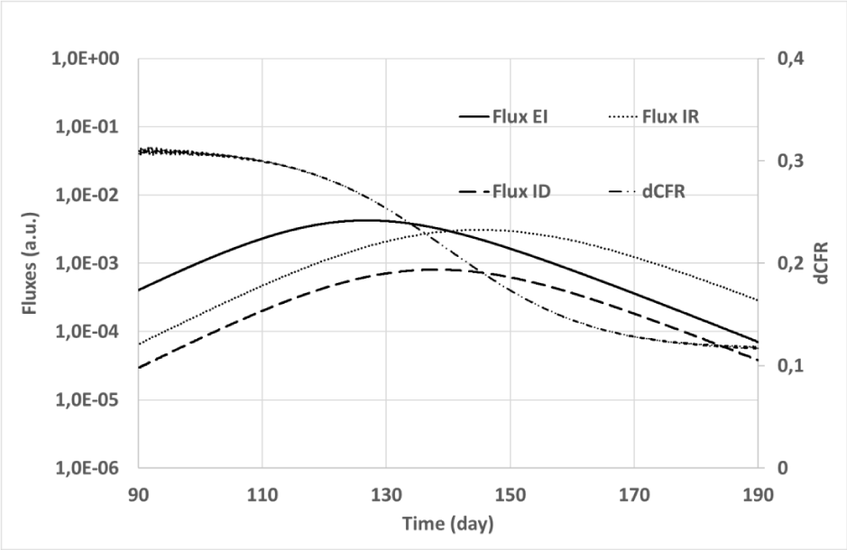
The simulation outputs are summarized in Figures 3, 4, and 5. Figure 3 shows the time evolution of classes of both the convolutional and the SIR models. Ratios of corresponding classes of the two models are plotted versus time in Figure 4, while Figure 5 depicts the input ( ${\text{Φ}}_{ei}\left(t\right)$ ) and output ( ${\text{Φ}}_{ir}\left(t\right),{\text{Φ}}_{id}\left(t\right)$ ) fluxes of class i(t), together with the dynamic estimate of the Case Fatality Rate (dCFR), which was calculated as:

Figure 3: Simulation #2: Time evolution of classes in the epidemy simulated with the convolutional (solid lines) and the SIR (dashed lines) models.

Figure 4: Simulation #2: Time evolution of new model to SIR model class ratios. Solid line: s(t) to SIR s(t) class ratio; dashed line: e(t) to SIR i(t) class ratio; Dot-dashed line: r(t) to SIR r(t) class ratio; Dotted line: i(t) to SIR i(t) class ratio.

Figure 5: Simulation #2: Fluxes and dynamic CFR vs time for the convolutional model. Solid line: flux Φei (t) from exposure to infected class; Dashed line: flux Φid (t) from infected to dead class; Dotted line: flux Φir (t) from infected to recovered class; Dot-Dashed line: dynamic Case Fatality Ratio (right vertical axis). The left vertical axis (fluxes) is plotted with a logarithmic scale.

$dCFR=\frac{{\text{Φ}}_{id}\left(t\right)}{{\text{Φ}}_{ir}\left(t\right),+{\text{Φ}}_{id}\left(t\right)}\text{ (24)}$

Let us note that fluxes ( ${\text{Φ}}_{ir}\left(t\right),{\text{Φ}}_{id}\left(t\right)$ ) are proportional to the number of outcomes in the corresponding compartments within a short time interval, hence it is the dynamic (instantaneous) value of the CFR estimate defined as deaths/(deaths + recovered) that is adopted often [28,37]. We also note that the exposed category e(t) rarely is traced precisely, so the death rate is often estimated considering the outcomes of the infected class only disregarding the flux ${\Phi }_{er}\left(t\right)$ .

Figures 3 and 4 demonstrate that the signals originated by the convolutional model are significantly delayed with respect to those calculated by the SIR model with the same R₀. Due to its structure, the convolutional model foresees important trouble encountered when facing the Covis-19 epidemy: when the disease becomes apparent, i.e.: i(t) assumes non-negligible values and patient hospitalization begins to grow, the class e(t) already is significantly diffused reducing the possibility to restrain the epidemy. Moreover, the convolutional model exhibits a significant persistence of i(t) and e(t)signals after the epidemy peak that is not found with the SIR. This point is evident in Figure 4 where the ratio between the signals e(t) and SIR i(t) significantly grows for large t. In other words, the convolutional model does not exhibit a sharp epidemy stopping, the simulated epidemic wave slowly vanishes away after the peak, and a tiny fraction of the population remains infectious for a long time.

Figure 5 shows that the ${\Phi }_{id}\left(t\right)$ flux toward the d(t) class (dashed line) resulting from simulations is larger in the initial phase of the simulated COVID-19 epidemy than near its termination when the predominant flux ${\text{Φ}}_{ir}\left(t\right)$ (dotted line) is toward the r(t) class. In the epidemic terminating phase ${\text{Φ}}_{ir}\left(t\right)$ is almost one order of magnitude greater than ${\text{Φ}}_{id}\left(t\right)$ , while at the beginning the simulated fluxes are comparable. The dCFR plot confirms this property that has been obtained with intrinsically constant mortality of the simulated epidemy. From a mathematical standpoint, the apparent reduction of infection gravity with increasing time is a direct consequence of the circumstance that the healing time $T_{ir}$ is on average greater than the dying time $T_{id}$ . As a rule of thumb, the apparent dynamic recovery rate of class i(t) at time is proportional to ${\Phi }_{ei}\left(t-T_{ir}\right)$ , while the dynamic death rate depends on the input flux ${\Phi }_{ei}\left(t-T_{id}\right)$ . If $T_{ir}\ge T_{id}$ , a greater death rate with rarer recoveries will appear near the epidemy beginning with respect to its conclusion.

A similar phenomenon has been observed in China where “the overall CFR was higher in the early stages of the outbreak” [33], and its origin still is debated [28]. Comparisons among the case-fatality rates in China, Italy, and other countries [40,41] showed a partially unexplained higher mortality of the COVID-19 epidemic in Italy. However, the data analyzed in [40] were sampled in the initial phase of the epidemic wave in Italy and near the top of the epidemy in China. Simulations performed with the convolutional model (Figure 5) suggest that the disparity of sampling time could imply a large difference in the apparent death rate, so the differences revealed by these works [28,33,40,41] might reflect the property $T_{ir}>T_{id}$ rather than possible differences in epidemy management or clinical response between the countries.

It is worth noting that recent virus epidemics have shown time-varying CFRs as reported in [42]. The SARS epidemy in 2003 was found to have an increasing CFR, lesser in the initial phase of the epidemic wave with respect to its conclusion [43]. We point out that the convolutive mathematical modeling discussed in this work can predict this characteristic by choosing $T_{ir}<T_{id}$ , i.e.: a recovering time on average shorter than the time to death.

Simulation #3

In this Section, we show the aggregate outcomes of several simulations with many combinations of the model-free parameters, all with γ = 0. We have investigated the criterion for epidemy spontaneous stopping and the asymptotic value as a function of $R_0$ .

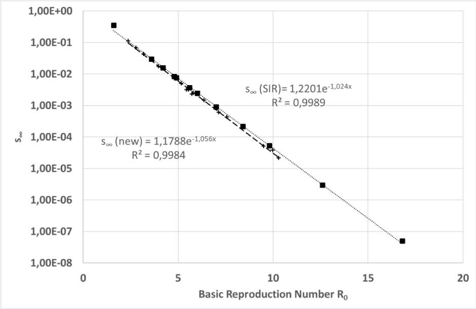
For both the examined models (convolutional and SIR), it was possible to find a clear link between the asymptotic value $s_{\infty }$ and the $R_0$ imposed on the simulations, as shown in Figure 6 and in Eq. (25).

Figure 6: Simulation #3: Asymptotic value of the susceptible class simulated for several combinations of free model parameters plotted versus the basic reproduction number. The vertical axis has a logarithmic scale.

$s_{\infty }\cong C{e}^{-a{R}_0}\text{ (25)}$

Where C and $a$ are positive constants that assume values close to one (best fit). Figure 6 clearly shows how carefully the relationship of Eq. (25) predicts the asymptotic limit $s_{\infty }$ of the susceptible class with a correlation coefficient greater than 0.99.

Substituting into Eq. (25) the limit $\underset{t\to +\infty }{\lim }s\left(t\right)$ from Eqs. (17) it is possible to find a simple relationship between function p(t) and R₀, as shown in the next equations.

$\underset{t\to +\infty }{\lim }s\left(0\right)e^{-p\left(t\right)}\cong C{e}^{-a{R}_0}$

$\underset{t\to +\infty }{\lim }p\left(t\right)=2k{\int }_o^{\infty }\frac{\left[\epsilon e\left(\tau \right)+i\left(\tau \right)\right]}{{\left[1-d\left(\tau \right)\right]}^2}d\tau \cong a{R}_0+\ln \frac{C}{s\left(0\right)}\approx R_0+0.182\text{ (26)}$

It is easy showing that the SIR model closely obeys the same equation:

$\underset{t\to +\infty }{\lim }p\left(t\right)=k{\int }_o^{\infty }i\left(\tau \right)d\tau \cong a{R}_0+\ln \frac{C}{s\left(0\right)}\approx R_0+0.182\text{ (27)}$

Integrals in Eqs. (26,27) can be considered as a measure of the epidemy “strength”, thus these equations show how the impact of an epidemy depends on a few parameters such as R₀, k and s(0)

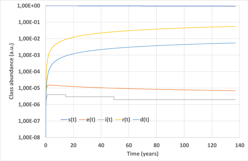
It is believed that an epidemy does not break out if R0<1, and that it stops when its basic reproduction number falls below 1 [44]. For the convolutional model, these properties seem untrue, and epidemy can survive for years although with vanishing rates. This circumstance is depicted in Figure 7, where class abundances are plotted versus time for an epidemic simulation characterized by R0= 0.946429, $\epsilon =k=0.16$ , $\alpha =\beta =0.7$ , $\gamma =0.0$ , $T_e=T_{ir}=T_{id}=T_r=6$ and ${\sigma }_e={\sigma }_{ir}={\sigma }_{id}={\sigma }_r=4$ . As can be seen, the convolutional model foresees a tiny-amplitude epidemic wave that propagates over years with almost vanishing e(t) and i(t) time derivatives, as dictated by Eqs. (13,14). This behavior should be ascribed to the delay and spreading of the output signals typical of the convolutive model: Delay allows e(t) and i(t) to grow even with a small R₀ while spreading prevents their fast zeroing. We note that the role of R₀ as epidemy stopping threshold seems untrue also for different epidemic models containing nonlinear terms [24].

Figure 7: Simulation #3: Time evolution of the epidemy simulated over a long time interval with the convolutional model.

The characteristics discussed above are relevant to developing strategies for epidemy mitigation or control.

Conclusions

We have shown the structure of a new epidemic model holding five population compartments, which introduces the concept of population fluxes among different classes. In the mathematical construction of the model, classes are considered time-invariant linear systems that connect the input to output fluxes by the convolution of the input flux with an IRF. The convolution with the normalized IRF introduces delay and spreading in the related class transition that can be thought of as a probabilistic temporal evolution of the epidemy. This mathematical structure guarantees that people leave a given class according to a lifelike temporal scheme (the IRF) starting from the time at which the same individuals entered the concerned class. The convolutional model does not adopt the unrealistic exponential decay, implicitly accepted by most deterministic models to compute the exit rate of a given compartment.

The model includes healthy carrier contribution to epidemy propagation, the option for recovered people to become newly susceptible, several free parameters that govern pathogen transmissibility, and time delay and spreading for any class transition admitted. The model can be useful to simulate the evolution of different types of epidemics and seems to be able to predict important features of the COVID-19 pandemic.

The performed analyses pointed out the following properties.

1. The convolutional model foresees important trouble encountered when facing the Covis-19 epidemy: when class i(t) assumes non-negligible values and patient hospitalization begins to grow, the class e(t) already is significantly diffused, reducing the possibility to restrain the epidemy.
2. Epidemic waves simulated with the convolutive modeling are significantly delayed in comparison with those calculated by the SIR model.
3. The convolutional model can predict the formation of epidemic oscillatory patterns for simulations in which recovered people can become newly susceptible to losing their immunization.
4. The new model admits a quasi-stationary regime in which the decrease of s(t) is continuously absorbed by the restored and deceased classes with vanishing derivatives of e(t) and i(t).
5. The new model allows a tiny epidemic wave to propagate for a long time even when .
6. The dynamic fatality rate of COVID-19 deduced from simulations performed with the convolutive model appears to be greater at epidemy beginning than in its stopping phase, a model property that can justify measured epidemiological data (behaviors) that recent investigations were unable to explain. According to the convolutional model, this epidemic property is the result of a long average recovering time . The convolutive model is even able to account for a CFR that apparently increases with increasing time, as in the case of SARS, a feature that would require the adoption of .
7. We have defined a quadrature function p(t) whose asymptotic limit determines the epidemy strength (i.e.: its impact on the population) and which roughly matches the value  R0 at epidemy beginning. We were able to find this quadrature function for both the convolutive and the SIR models.

Points 4 and 5 are less important per se, as their effects can be quite small from an epidemic point of view, but they prove the inexistence of a sharp epidemy stopping option. They indeed demonstrate that epidemics like COVID-19 can silently propagate over years even involving tiny fractions of the population whenever $R_t\le 1$ , but being able to spring off every time the basic reproduction number rise.

The features outlined above should be carefully considered when planning strategies for epidemy mitigation or control.

1. Satorras RP, Castellano C, Mieghem VP, Vespignani A. Epidemic processes in complex networks, Reviews of Modern Physics. 2015; 87: 925. DOI:https://doi.org/10.1103/RevModPhys.87.925
2. Koher A, Hartmut Lentz HK, Gleeson JP, Hövel P. Contact-Based Model for Epidemic Spreading on Temporal Networks, Physical Review X. 2019; 9: 031017.
3. Gumel AB, Ruan S, Day T, Watmough J, Brauer F, van den Driessche P, Gabrielson D, Bowman C, Alexander ME, Ardal S, Wu J, Sahai BM. Modelling strategies for controlling SARS outbreaks. Proc Biol Sci. 2004 Nov 7;271(1554):2223-32. doi: 10.1098/rspb.2004.2800. PMID: 15539347; PMCID: PMC1691853.
4. Calafiore GC, Novara C, Possieri C. A time-varying SIRD model for the COVID-19 contagion in Italy. Annu Rev Control. 2020;50:361-372. doi: 10.1016/j.arcontrol.2020.10.005. Epub 2020 Oct 26. PMID: 33132739; PMCID: PMC7587010.
5. Tang Z, Li X, Li H. Prediction of New Coronavirus Infection Based on a Modified SEIR Model, medRxiv preprint. 2020. doi: https://doi.org/10.1101/2020.03.03.20030858.
6. Gumel AB, McCluskey CC, Watmough J. An sveir model for assessing potential impact of an imperfect anti-sars vaccine. Math Biosci Eng. 2006 Jul;3(3):485-512. doi: 10.3934/mbe.2006.3.485. PMID: 20210376.
7. Huang G, Takeuchi Y, Ma W, Wei D. Global stability for delay SIR and SEIR epidemic models with nonlinear incidence rate. Bull Math Biol. 2010 Jul;72(5):1192-207. doi: 10.1007/s11538-009-9487-6. Epub 2010 Jan 21. PMID: 20091354.
8. Wang WD. Global behavior of an SEIRS epidemic model with time delays. Appl Math Lett. 2002; 15:423–428.
9. Buonomo B, Cerasuolo M. The effect of time delay in plant--pathogen interactions with host demography. Math Biosci Eng. 2015 Jun;12(3):473-90. doi: 10.3934/mbe.2015.12.473. PMID: 25811557.
10. Goel K, Nilam. A mathematical and numerical study of a SIR epidemic model with time delay, nonlinear incidence and treatment rates. Theory Biosci. 2019 Nov;138(2):203-213. doi: 10.1007/s12064-019-00275-5. Epub 2019 Jan 21. PMID: 30666514.
11. Kumar A, Nilam. Mathematical analysis of a delayed epidemic model with nonlinear incidence and treatment rates. J Eng Math. 2019; 115(1):1–20.
12. Li M, Liu X. An SIR epidemic model with time delay and general nonlinear incidence rate. Abstr Appl Anal 2014. Article ID 131257.
13. Naresh R, Tripathi A, Tchuenche JM, Sharma D. Stability analysis of a time delayed SIR epidemic model with nonlinear incidence rate. Comput Math Appl. 2009; 58:348–359.
14. Din A, Li Y, Khan T, Zaman G. Mathematical analysis of spread and control of the novel corona virus (COVID-19) in China. Chaos Solitons Fractals. 2020 Dec;141:110286. doi: 10.1016/j.chaos.2020.110286. Epub 2020 Sep 23. PMID: 32989346; PMCID: PMC7510499.
15. McCluskey CC. Complete global stability for an SIR epidemic model with delay - Distributed or discrete, Nonlinear Analysis: Real World Applications. 2010; 11: 55-59.
16. Beretta E, Hara T, Ma W, Takeuchi Y. Global asymptotic stability of an SIR epidemic model with distributed time delay, Nonlinear Analysis. 2001; 47: 4107-4115.
17. Takeuchi Y, Ma W, Beretta E. Global asymptotic properties of a delay SIR epidemic model with finite incubation times, Nonlinear Analysis. 2000; 42: 931–947.
18. Benavides EM. Robust predictive model for Carriers, Infections and Recoveries (CIR): predicting death rates for COVID-19 in Spain. arXiv. 2020; 2003.13890v2.
19. Cui Q, Qiu Z, Liu W, Hu Z. Complex dynamics of an SIR epidemic model with nonlinear saturated incidence rate and recovery rate. Entropy. 2017. https://doi.org/10.3390/e19070305.
20. Dubey B, Dubey P, Dubey US. Dynamics of a SIR model with nonlinear incidence rate and treatment rate. Appl Appl Math. 2015; 2(2):718-737.
21. Korobeinikov A, Maini PK. Non-linear incidence and stability of infectious disease models. Math Med Biol. 2005 Jun;22(2):113-28. doi: 10.1093/imammb/dqi001. Epub 2005 Mar 18. PMID: 15778334.
22. Liu WM, Levin SA, Iwasa Y. Influence of nonlinear incidence rates upon the behavior of SIRS epidemiological models. J Math Biol. 1986;23(2):187-204. doi: 10.1007/BF00276956. PMID: 3958634.
23. Xu R, Ma Z. Stability of a delayed SIRS epidemic model with a nonlinear incidence rate. Chaos Solut Fractals. 2009; 41:2319-2325.
24. Li GH, Zhang YX. Dynamic behaviors of a modified SIR model in epidemic diseases using nonlinear incidence and recovery rates. PLoS One. 2017 Apr 20;12(4):e0175789. doi: 10.1371/journal.pone.0175789. PMID: 28426775; PMCID: PMC5398581.
25. Din A, Li Y, Muhammad Khan F, Ullah Khan Z, Liu P. On Analysis of fractional order mathematical model of Hepatitis B using Atangana–Baleanu Caputo (ABC) derivative, Fractals. 2021; 2240017. DOI: 10.1142/S0218348X22400175
26. Din A, Li Y, Yusuf A, Isa Ali A. Caputo type fractional operator applied to Hepatitis B system, Fractals. 2021. DOI: 10.1142/S0218348X22400230
27. Nadler P, Wang S, Arcucci R, Yang X, Guo Y. An epidemiological modelling approach for COVID-19 via data assimilation. Eur J Epidemiol. 2020 Aug;35(8):749-761. doi: 10.1007/s10654-020-00676-7. Epub 2020 Sep 4. PMID: 32888169; PMCID: PMC7473594.
28. Iosa M, Paolucci S, Morone G. COVID-19: A Dynamic Analysis of Fatality Risk in Italy. Front Med (Lausanne). 2020 Apr 30;7:185. doi: 10.3389/fmed.2020.00185. PMID: 32426362; PMCID: PMC7203466.
29. Kermack WO, McKendrick AG. A contribution to the mathematical theory of epidemics, Proceedings of the Royal Society of London A: Mathematical, Physical and Engineering Sciences. The Royal Society. 1927; 115(772): 700-721.
30. Kaddar A. On the Dynamics of a Delayed Sir Epidemic Model with a Modified Saturated Incidence Rate, Electronic Journal of Differential Equations. 2009; 2009: 133; 1-7: 1072-6691. URL: http://ejde.math.txstate.edu or http://ejde.math.unt.edu
31. Diekmann O, Heesterbeek JA, Metz JA. On the definition and the computation of the basic reproduction ratio R0 in models for infectious diseases in heterogeneous populations. J Math Biol. 1990;28(4):365-82. doi: 10.1007/BF00178324. PMID: 2117040.
32. Mazurkin PM. Waves of the dynamics of the rate of increase in the parameters of COVID-19 in Russia for 03/25/2020-12/31/2020 and the forecast of all cases until 08/31/2021. Ann Math Phys. 2021; 4(1): 048-065. DOI: https://dx.doi.org/10.17352/amp.000024
33. WHO. Report of the WHO-China Joint Mission on Coronavirus Disease 2019 (COVID-19). Feb, 2020. https://www.who.int/docs/defaultsource/coronaviruse/who-china-jointmission-on-COVID-19-final-report.pdf (accessed on May 23, 2020).
34. Backer JA, Klinkenberg D, Wallinga J. Incubation period of 2019 novel coronavirus (2019-nCoV) infections among travellers from Wuhan, China. 2020; 20–28 January 2020. Euro Surveill; 25, 2000062.
35. Li Q, Xuhua G, Wu P, Wang X. Early Transmission Dynamics in Wuhan, China, of Novel Coronavirus–Infected Pneumonia, New England Journal of Medicine. 2020; 382: 1199-1207. DOI: 10.1056/NEJMoa2001316
36. Zhou T, Liu Q, Yang Z, Liao J, Yang K, Bai W, Lu X, Zhang W. Preliminary prediction of the basic reproduction number of the Wuhan novel coronavirus 2019-nCoV. J Evid Based Med. 2020 Feb;13(1):3-7. doi: 10.1111/jebm.12376. Epub 2020 Feb 12. PMID: 32048815; PMCID: PMC7167008.
37. Baud D, Qi X, Nielsen-Saines K, Musso D, Pomar L, Favre G. Real estimates of mortality following COVID-19 infection. Lancet Infect Dis. 2020 Jul;20(7):773. doi: 10.1016/S1473-3099(20)30195-X. Epub 2020 Mar 12. PMID: 32171390; PMCID: PMC7118515.
38. Palmieri L, Andrianou X, Bella A, Bellino S. Characteristics of COVID-19 patients dying in Italy. 2020. Istituto Superiore di Sanità. https://www.epicentro.iss.it/coronavirus/bollettino/Report-COVID-2019_20_marzo_eng.pdf
39. Palmieri L, Andrianou X, Barbariol P, Bella A, Bellino S. Caratteristiche dei pazienti deceduti positivi all’infezione da SARS-CoV-2 in Italia - Dati al 21 maggio 2020, Istituto Superiore di Sanità. 2020. https://www.epicentro.iss.it/coronavirus/bollettino/Report-COVID-2019_21_maggio.pdf
40. Onder G, Rezza G, Brusaferro S. Case-Fatality Rate and Characteristics of Patients Dying in Relation to COVID-19 in Italy. JAMA. 2020 May 12;323(18):1775-1776. doi: 10.1001/jama.2020.4683. Erratum in: JAMA. 2020 Apr 28;323(16):1619. PMID: 32203977.
41. Ergönül Ö, Akyol M, Tanrıöver C, Tiemeier H, Petersen E, Petrosillo N, Gönen M. National case fatality rates of the COVID-19 pandemic. Clin Microbiol Infect. 2021 Jan;27(1):118-124. doi: 10.1016/j.cmi.2020.09.024. Epub 2020 Sep 23. PMID: 32979575; PMCID: PMC7510430.
42. Kim DH, Choe YJ, Jeong JY. Understanding and Interpretation of Case Fatality Rate of Coronavirus Disease 2019. J Korean Med Sci. 2020 Mar 30;35(12):e137. doi: 10.3346/jkms.2020.35.e137. PMID: 32233163; PMCID: PMC7105506.
43. Venkatesh S, Memish ZA. SARS: the new challenge to international health and travel medicine. East Mediterr Health J. 2004 Jul-Sep;10(4-5):655-62. PMID: 16335659.
44. van den Driessche P, Watmough J. Reproduction numbers and sub-threshold endemic equilibria for compartmental models of disease transmission. Math Biosci. 2002 Nov-Dec;180:29-48. doi: 10.1016/s0025-5564(02)00108-6. PMID: 12387915.