The behavior of population dispersion employing various numerical techniques

The exploration of population diversity motivated us to present this paper. A mathematical model for the ecological process of population dispersion is finally considered by us to figure out the dispersion of population along the area. The dispersal from one's home site to the next is considered the most important phenomenon in the demographic and evolutionary dynamics of the population. The most important factor regarding dispersal is the spatial distribution of individuals. This dispersal may result in enhanced clamping, huge randomness, or even more spacing. The Adomian Decomposition method has opted to work out the problem analytically. Numerical schemes brought an approximate solution by incorporating the Forward-in-Time and Central-In-Space (FTCS) scheme, the Crank Nicolson (CN) scheme, and Numerov’s method. The validity and efficiency of schemes employed for the proposed model are supported by core properties like stability, consistency, and convergence. A comparison is made between the results calculated via schemes and the one analytically.

Introduction

Molecular, cell, or organism populations are seldom evenly distributed over a featureless environment, with some interest in their motions, migrations, and redistributions at the level of the people’s movement may be the results of the special mechanochemical process from muscle macroscopic contractions or the streaming of amoeboids. At the level of the population, these various mechanisms may have less bearing on migration than on the degree of overcrowding and movement of the fluid or air in which the organisms live. It is often appropriate to make a continuum assumption on the collective level that is, to depict discrete cells or organisms through continuous distributions of density. This leads to partial differential equations that are quite often analogous to traditional models for diffusions, convections, or attraction by molecules. Biological models involving Partial Differential Equations (PDEs) historically date back to the work of K. Pearson and the Blake man at the start of the 1900s. In 1930 there were others including R.A Fisher who applied PDEs for the spatial diffusions of genes and diseases. A significant aspect of many living organisms is the capability to grow up in size while sustaining a scrupulous shape or geometry. This possession is common in advanced multicellular organisms where well-built intercellular communication bonds are present. It also happens in much more primal locales such as populations of microorganisms, although the underlying mechanisms might be rather different. Here we consider the nutrient-dependent growth of toadstool cells and conclude whether a colony can demonstrate time spread over space. Focusing on the growth of yeast under standard laboratory conditions, a distinctive experiment initiates with a Petri dish having a small volume of sterile nutrient-rich medium. Generally, the medium is a solidified gel-like material called agar, which allows the liberated diffusion of tiny molecules and provides a convenient two-dimensional surface on which to grow micro-organisms. A little number of yeast cells is left on the agar surface. After absorption of nutrients from below, they grow and multiply to such an extent that the population gradually enlarges and spreads over the surface of the substrate. In a number of cases, the shape of the colony remains essentially fixed as it grows in size. Gray and Kirwan [1] established a model for the spread of yeast colonies which, with some modifications, will serve as our example. A colony of yeast usually takes the form of a shiny disk, visible to the naked eye that continually enlarges in diameter.

PDEs have several applications in fields like engineering, biology, chemistry, game theory, and many more. These are proficient tools to frame the diverse problems mathematically emerging in different fields of study. Diffusion is a process through which matter is transferred from one part of the material to the other part. Diffusion equations can be used to model such a natural phenomenon in which there is a clear transference of particles or molecules from one place to the other. One such model was proposed by Skellem in 1951. He was the first to show the population diversity of flora and fauna in the form of PDEs [2-8]. Such kinds of PDEs are solved analytically, and numerically using MATLAB. For the solution of the selected model, we use a well-known semi-analytical method known as the Adomian Decomposition method created by George Adomian (1970-1990) [2,3]. In the past several numerical methods are developed to solve PDEs, linear as well as nonlinear using implicit and explicit techniques [15-20]. In [33] authors present a robust (t, n) threshold version which is efficient as well, for Schnorr’s signature scheme. In [34] authors construct and investigate the two-step scheme for the

Schrödinger equation [35]. Deals with the initial-boundary value problem for the 1D time dependent Schrödinger equation on the half-axis [36]. Deals with an initial-boundary value problem for a 2D time-dependent Schrödinger equation. In [37] numerical stability in reference to mathematical analysis is brought under discussion [38]. Provides rich information on computational fluid dynamics covering several numerical techniques. Three finite difference implicit schemes are used in [39] which are unconditionally stable. In [40] authors evaluate bird populations in A doğan La es by statistical means of Poisson and negative binomial regression models.

One of the most broadly used techniques is FTCS. This technique is conditionally stable. This scheme can be used to solve PDEs numerically. Certain implicit schemes are efficiently used, and such schemes are unconditionally stable. One such scheme is built by John Crank and Phyllis Nicolson. In this scheme for each time step, we have to use a system of equations for a linear problem. For nonlinear problems, the obtained system of equations is tridiagonal which can be solved firstly by TMA (Tridiagonal Matrix Algorithm). Instead of calculating the whole matrix, this method has the advantage of speedy calculations.

In the present work, we have provided a numerical investigation of the population dispersion model via several numerical techniques. These include FTCS (Forward in time and central in space) scheme, the Crank-Nicolson method, and Numerov’s method. The analysis of the applied schemes is also provided which includes stability, consistency, and accuracy. The solution’s uniqueness is discussed theoretically. The diffusion coefficient is discussed through plots in detail. Moreover, a comparison among the schemes is provided in the form of a table. The selected model is

$\frac{\partial p}{\partial t}=D\frac{{\partial }^{2}p}{\partial x^2}+\alpha p\text{ (1)}$

This equation efficiently presents the spread of populations over an area dynamically. Here p (x, t) denotes the population at some location x at time t, α is the rate of growth of the considered population and D is taken as the dispersion coefficient [4-8].

$p(x,0)=\delta (x)\text{ (2)}$

Where δ (x) represents the Dirac Delta function.

The setting of the paper is as follows: In this section, we present the analytical solution of (1) using (2). In section 2 we present numerical techniques like FTCS, Crank Nicolson, and Numerov’s method. The characteristics like stability, consistency, and accuracy are discussed in the same section. In the following sections, we presented the results of employed schemes.

To initiate our analysis, we first rephrase (1) in an operator shape as

$L_t(p)=D{L}_{xx}(p)+\alpha p\text{ (3)}$

Where differential operators are defined as under

$L_t=\frac{\partial }{\partial t}and{L}_x=\frac{{\partial }^2}{\partial x^2}\text{ (4)}$

Integral operators $L_t{}^{-1}\text{and}{L}_x{}^{-1}$ can take the form

$L_t{}^{-1}(.)={\displaystyle \underset{0}{\overset{t}{\int }}(.)dt,L_x{}^{-1}}(.)={\displaystyle \iint (.)dxdx}\text{ (5)}$

It means that

$L_t{}^{-1}{L}_{t}p\left(x,t\right)=p\left(x,t\right)-p\left(x,0\right)\text{ (6)}$

Apply $L_t{}^{-1}$ on both sides of (3) and use the initial condition

$p\left(x,t\right)=f\left(x\right)+L_t{}^{-1}\left(L_{x}p\left(x,t\right)\right)\text{ (7)}$

Now we find unknown functions P (x,t) as the sum of components and are defined by series like

$p\left(x,t\right)={\displaystyle \sum _{n=0}^{\infty }{p}_n}\left(x,t\right)\text{ (8)}$

After finding components P₀,P₁,…. and setting the values in (7) leads to

${\displaystyle \sum _{n=0}^{\infty }{p}_n}\left(x,t\right)=f\left(x\right)+L_t{}^{-1}\left(L_x\left({\displaystyle \sum _{n=0}^{\infty }{p}_n}\left(x,t\right)\right)\right)\text{ (9)}$

$p_0+p_1+p_2+\mathrm{...}=f\left(x\right)+L_t{}^{-1}\left(L_x\left(p_0+p_1+\mathrm{...}\right)\right)\text{ (10)}$

Here

$p_0\left(x\right)=\delta \left(x\right)$

$p_1\left(x\right)=\left(\alpha \delta \left(x\right)+D{\delta }^{″}\left(x\right)\right)t$

$p\left(x,t\right)=\frac{{\stackrel{⌢}{p}}_0}{2{\left(\pi Dt\right)}^{1/2}}{e}^{\alpha t-\frac{x^2}{4Dt}}\text{ (11)}$

Numerical methods

We purport a finite domain ω for the numerical computation of (1). We exhibit a rectangular mesh M to discretize the partial differential equation. Spatial coordinates are considered while time coordinates are presented vertically. Assume x_i = a+(i-1h) where i = 1,2,3,…. and a is the left-hand boundary, t_n = nk where n = 1,2,3,….. We represent the approximate and exact solution at each nodal point (x_i,t_n) $p^n{}_{i}and{P}_i{}^n$ respectively. In many textbooks, the numeric solution of the population equation is discussed, for instance, Ames [9,10],

Forward time-centered space scheme

The finite difference method can be applied to obtain an approximate solution of (1). In all numerical solutions, the PDEs are converted into a discrete approximation. The discrete word in this context indicates that a numerical solution is known in the physical domain just at a finite number of points. The numerical method user can choose the number of those points. Generally, an increment in the number of nodes not only results in the increment of the resolution (i.e., detail), but it enhances the accuracy of the numerical computation. The discrete estimation provides a set of algebraic equations that are computed for unknown values. The mesh represents the set of positions where the discrete solution is calculated. These points are termed nodes, and if one were to sketch lines sandwiched between adjacent nodes in the domain, the consequential image would bear a resemblance to a net or mesh. Two key parameters of the net are ∆x the local adjacent distance between points in space and ∆t indicate the local distance between adjacent time steps. The straightforward examples considered in this item, ∆x and ∆t are regarded as uniform all the way through the mesh. The gist idea of the FD method is to replace continuous derivatives with so-called difference formulas that engage only the discrete values associated with positions on the mesh [11-15].

Consider

$p=p^n{}_i\text{ (12)}$

$p_t=\frac{p^{n+1}{}_i-p^n{}_i}{\Delta t}\text{ (13)}$

$p_{xx}=\left(\frac{p^n{}_{i+1}-2p^n{}_i+p^n{}_{i-1}}{\Delta x^2}\right)\text{ (14)}$

The substitution of the above results (12-14) in the following

$\frac{p^{n+1}{}_i-p^n{}_i}{\Delta t}=D\left(\frac{p^n{}_{i+1}-2p^n{}_i+p^n{}_{i-1}}{\Delta x^2}\right)+\alpha p^n{}_i$

$p^{n+1}{}_i=p^n{}_i+D\Delta t\left(\frac{p^n{}_{i+1}-2p^n{}_i+p^n{}_{i-1}}{\Delta x^2}\right)+\alpha \Delta t{p}^n{}_i\text{ (15)}$

Where $R_1=\frac{D\Delta t}{\Delta x^2}$ . After some simplification we get

$p^{n+1}{}_i=p^n{}_i\left(1-2R_1+\alpha \Delta t\right)+R_1\left(p^n{}_{i+1}+p^n{}_{i-1}\right)\text{ (16)}$

Stability, consistency and accuracy

An FD scheme is considered stable if the computational error reduces as the calculation progressed from one marching step to the next step.

An FD scheme is called consistent if by decreasing the mesh and time step size, the truncation error tends to zero.

Stability of forward time-centered space scheme: We want to study the condition for which the error can be identified. Numerous techniques can be employed to discover the stability; here we use Vonn Neumann stability analysis. Let us assume

$p^n{}_i=e^{\alpha nk}{e}^{\lambda \beta ih}\text{ (17)}$

Where $\lambda =\sqrt{-1}$ , Consider

$p_i{}^{n+1}=p_i{}^n\left(1-2R_1+R_2\right)+R_1\left(p_i{{}_{+1}}^n-p_{i-1}{}^n\right)\text{ (18)}$

Substitution results in

$e^{\alpha k}=\left(1-2R_1+R_2\right)+R_1\left(e^{\lambda \beta h}+e^{-\lambda \beta h}\right)\text{ (19)}$

After some simplification we get

$e^{\alpha k}=\left(1-2R_1+R_2\right)+R_1\left(2\cos \beta h\right)\text{ (20)}$

For stability $\left|e^{\alpha k}\right|\le 1$

$\left|1-2R_1+R_2+2R_1\cos \beta h\right|\le 1\text{ (21)}$

Solving this leads us to

$4R_1\ge R_2\text{ (22)}$

Consistency of forward time-centered space scheme:

For consistency, we define an operator as follows

$L=\frac{\partial }{\partial t}-D\frac{{\partial }^2}{\partial x^2}-\alpha \text{ (23)}$

Where

$L_p=\frac{\partial p}{\partial t}-D\frac{{\partial }^{2}p}{\partial x^2}-\alpha p\text{ (24)}$

After some simplification, we obtain

$L^n{}_{i}p=\frac{p^{n+1}{}_i-p^n{}_i}{\Delta t}-D{p}_{xx}=\left(\frac{p^n{}_{i+1}-2p^n{}_i+p^n{}_{i-1}}{\Delta x^2}\right)-\alpha p\text{ (25)}$

$L^n{}_i=\frac{\Delta t\frac{\partial p}{\partial t}+{(\Delta t)}^2\frac{{\partial }^{2}p}{\partial t^2}}{\Delta t}-D\left(\frac{{(\Delta x)}^2\frac{{\partial }^{2}p}{\partial x^2}}{\Delta x^2}\right)-\alpha p\text{ (26)}$

$L^n{}_i-L^n{}_{i}p=-(\Delta t)\frac{{\partial }^{2}p}{\partial t^2}\text{ (27)}$

When $\Delta t,\Delta x\to 0$

We get $L^n{}_i-L^n{}_{i}p\to 0$

So FTCS scheme is consistent.

Accuracy of forward time-centered space scheme:

To analyze the accuracy of the FTCS scheme for the population dynamics linear model, we apply the Taylor series term-wise by using equation (1) as follows

$\begin{array}{l}p\left(x,t+k\right)-p\left(x,t\right)-R_1\left(p\left(x+h,t\right)-2p\left(x,t\right)+p\left(x-h,t\right)-\alpha k\right);\\ p_t=k{p}_t+\frac{k^2}{2}{p}_{tt}+\frac{k^3}{6}{p}_{ttt}+\mathrm{...};\\ p_{tt}=h^2{p}_{xx}+h^4\frac{1}{12}{p}_{xxx}+\mathrm{...};\end{array}\}\text{ (28)}$

Putting values in the above equation, obtained results are

$\begin{array}{l}equation=\left(k{p}_t+\frac{k^2}{2}{p}_{tt}+\frac{k^3}{6}{p}_{ttt}+\mathrm{...}\right)-\frac{Dk}{h^2}\left(h^2{p}_{xx}+h^4\frac{1}{12}{p}_{xxx}.+\mathrm{..}\right)-k\alpha p;\\ equation=k\left(0\right)+k\left(p_{tt}+\frac{k^2}{2}{p}_{ttt}+\mathrm{...}\right)\end{array}\}\text{ (29)}$

$equation=k\left(\frac{k}{2}{p}_{tt}+\frac{k^2}{2}{p}_{ttt}-\frac{D{h}^2}{12}{p}_{xxx}+\mathrm{...}\right)\text{ (30)}$

This shows that the scheme is 1st order accurate in time and 2nd order in space.

Crank Nicolson Scheme

The FTCS and BTCS implicit schemes produce truncation errors in time having O(∆t)². For time-accurate solutions, the Crank-Nicolson scheme has a considerable advantage [16]. In addition, the Crank-Nicolson scheme is not significantly more difficult to put into operation than the BTCS scheme, and it has a temporal truncation error that is O(∆t)². The Crank-Nicolson scheme is implicit, like BTCS, and it also possesses unconditional stability [17-22].

Consider the following

$\begin{array}{l}{p}_t=\frac{p_i{}^{n+1}-p_i{}^n}{\Delta t}\\ p_{xx}=\left(\frac{p_i{{}_{+1}}^{n+1}-2p_i{}^{n+1}-p_{i-1}{}^{n+1}}{2\Delta x^2}\right)+\left(\frac{p_i{{}_{+1}}^n-2p_i{}^n-p_{i-1}{}^n}{2\Delta x^2}\right)\\ p_i=\left(\frac{p_i{}^{n+1}+p_i{}^n}{2}\right)\end{array}$

Putting these values in equation (1)

$\begin{array}{l}\frac{p_i{}^{n+1}-p_i{}^n}{\Delta t}=\frac{D}{2{\left(\Delta x\right)}^2}\left(p_i{{}_{+1}}^{n+1}-2p_i{}^{n+1}-p_{i-1}{}^{n+1}\right)+\left(p_i{{}_{+1}}^n-2p_i{}^n-p_{i-1}{}^n\right)+\alpha \left(\frac{p_i{}^{n+1}+p_i{}^n}{2}\right)\\ p_i{}^{n+1}\left(1+2F_1-F_2\right)-F_1{p}_i{{}_{+1}}^{n+1}-F_1{p}_{i-1}{}^{n+1}=F_1{p}_i{{}_{+1}}^n+p_i{}^n\left(-2F_1+F_2+1\right)+F_1{p}_{i-1}{}^n\end{array}$

$p_i{}^{n+1}-p_i{}^n=\frac{D\Delta t}{2{\left(\Delta x\right)}^2}\left(p_i{{}_{+1}}^{n+1}-2p_i{}^{n+1}-p_{i-1}{}^{n+1}\right)+\left(p_i{{}_{+1}}^n-2p_i{}^n-p_{i-1}{}^n\right)+\alpha \Delta t\left(\frac{p_i{}^{n+1}+p_i{}^n}{2}\right)$

$F_1=\frac{D\Delta t}{2{\left(\Delta x\right)}^2},F_2=\frac{\alpha \Delta t}{2}$

$p_i{}^{n+1}-p_i{}^n=F_1\left(p_i{{}_{+1}}^{n+1}-2p_i{}^{n+1}-p_{i-1}{}^{n+1}\right)+\left(p_i{{}_{+1}}^n-2p_i{}^n-p_{i-1}{}^n\right)+F_2\left(p_i{}^{n+1}+p_i{}^n\right)$

$p_i{}^{n+1}-p_i{}^n=F_1{p}_i{{}_{+1}}^{n+1}+p_i{}^{n+1}\left(-2F_1+F_2\right)+F_1{p}_{i-1}{}^{n+1}+F_1{p}_i{{}_{+1}}^n+p_i{}^n\left(-2F_1+F_2\right)+F_1{p}_{i-1}{}^n$

$p_i{}^{n+1}\left(1+2F_1-F_2\right)-F_1{p}_{i+1}{}^{n+1}-F_1{p}_{i-1}{}^{n+1}=F_1{p}_{i+1}{}^n+p_i{}^n\left(-2F_1+F_2+1\right)+F_1{p}_{i-1}{}^n\text{ (31)}$

Which is the final discretization?

Stability of crank Nicolson Scheme:

For stability, we consider (31)

$p_i{}^{n+1}\left(1+2F_1-F_2\right)-F_1{p}_i{{}_{+1}}^{n+1}-F_1{p}_{i-1}{}^{n+1}=F_1{p}_i{{}_{+1}}^n+p_i{}^n\left(-2F_1+F_2+1\right)+F_1{p}_{i-1}{}^n$

Where $F_1=\frac{D\Delta t}{2{(\Delta x)}^2},F_2=\alpha \Delta t$

Assume

$p^n{}_i=e^{\alpha nk}{e}^{\lambda \beta ih}\text{ (32)}$

$p^{n+1}{}_i=e^{\alpha (n+1)k}{e}^{\lambda \beta ih}\text{ (33)}$

$p^{n+1}{}_{i+1}=e^{\alpha (n+1)k}{e}^{\lambda \beta (i+1)h}\text{ (34)}$

$p^{n+1}{}_{i-1}=e^{\alpha (n+1)k}{e}^{\lambda \beta (i-1)h}\text{ (35)}$

$p^n{}_{i+1}=e^{\alpha (n)k}{e}^{\lambda \beta (i+1)h}\text{ (36)}$

$p^n{}_{i-1}=e^{\alpha (n)k}{e}^{\lambda \beta (i-1)h}\text{ (37)}$

Where $\lambda =\sqrt{-1}$

Taking into account (13) and after some simplification, we find that

$\left|e^{\alpha k}\right|=\left|\frac{F_1{e}^{\lambda \beta h}-(2F_1+F_2+1)+F_1{e}^{-\lambda \beta h}}{F_1{e}^{\lambda \beta h}+(-2F_1+F_2-1)+F_1{e}^{-\lambda \beta h}}\right|\text{ (38)}$

Obviously $\left|e^{\alpha k}\right|=1$

Hence Crank Nicolson scheme is unconditionally stable.

Consistency of Crank Nicolson Scheme:

For consistency we consider

$\begin{array}{l}{p}^{n+1}{}_{i+1}=p^n{}_i+\Delta t\frac{\partial p}{\partial t}+\Delta x\frac{\partial p}{\partial x}+\frac{1}{2}{\left(\Delta x\frac{\partial }{\partial x}+\Delta t\frac{\partial }{\partial t}\right)}^{2}p;\\ p^{n+1}{}_{i+1}=p^n{}_i+\Delta t\frac{\partial p}{\partial t}+\Delta x\frac{\partial p}{\partial x}+\frac{1}{2}\left(\Delta x^2\frac{{\partial }^{2}p}{\partial x^2}+\Delta t^2\frac{{\partial }^{2}p}{\partial t^2}+\Delta x\frac{\partial p}{\partial x}\Delta t\frac{\partial p}{\partial t}\right)\\ p^{n+1}{}_{i-1}=p^n{}_i+\Delta t\frac{\partial p}{\partial t}-\Delta x\frac{\partial p}{\partial x}+\frac{1}{2}\left(\Delta x^2\frac{\partial p^2}{\partial x^2}+\Delta t^2\frac{\partial p^2}{\partial t^2}-2\Delta x\frac{\partial p}{\partial x}\Delta t\frac{\partial p}{\partial t}\right);\end{array}\}\text{ (39)}$

Define the operator as

$\begin{array}{l}L=\frac{\partial }{\partial t}-D\frac{{\partial }^{2}p}{\partial x^2}-\alpha \\ L_p=\frac{\partial p}{\partial t}-D\frac{{\partial }^{2}p}{\partial x^2}-\alpha p\\ L^n{}_{i}p=\frac{p^{n+1}{}_i-p^n{}_i}{\Delta t}-\frac{D}{2{(\Delta x)}^2}\left(p_i{{}_{+1}}^{n+1}-2p_i{}^{n+1}-p_{i-1}{}^{n+1}\right)+\left(p_i{{}_{+1}}^n-2p_i{}^n-p_{i-1}{}^n\right)-\alpha \left(\frac{p_i{}^{n+1}+p_i{}^n}{2}\right)\end{array}\}\text{ (40)}$

Now

$\begin{array}{l}{L}_p-L^n{}_{i}p=\frac{\partial p}{\partial t}-D\frac{{\partial }^{2}p}{\partial x^2}-\alpha p-[\left(\frac{1}{\Delta t}\{\Delta t\frac{\partial p}{\partial t}+{(\Delta t)}^2\frac{{\partial }^{2}p}{\partial t^2}+\mathrm{...}\}\right)-\frac{D}{2{(\Delta x)}^2}\left(2\{\Delta t\Delta x^2\frac{\partial p}{\partial t}+{(\Delta t)}^2\frac{{\partial }^{2}p}{\partial t^2}+\mathrm{...}\}\right)\\ -D/2{(}^{\Delta }\{{(}^{\Delta }\frac{{\partial }^{2}p}{\partial x^2}-\frac{\alpha }{2}\{2p_i{}^n+\Delta t\frac{\partial p}{\partial t}+{(}^{\Delta }\frac{{\partial }^{2}p}{\partial t^2}+\mathrm{...}\}]\end{array}\}$

When

$\begin{array}{l}\Delta t,\Delta x\to 0\\ L_p-L^n{}_{i}p\to 0\text{ (41)}\end{array}$

Which leads to the consistency of the Crank-Nicolson scheme.

Accuracy of Crank Nicolson Scheme:

The Crank Nicolson Scheme applied at equation (1) can be written as

$u_i{}^{n+1}-p_i{}^n=\frac{D}{h{k}^2}\left(p_i{{}_{+1}}^{n+1}-2p_i{}^{n+1}-p_{i-1}{}^{n+1}+p_i{{}_{+1}}^n-2p_i{}^n-p_{i-1}{}^n\right)-\frac{\alpha k}{2}\left(p_i{}^{n+1}+p_i{}^n\right);\text{ (42)}$

Putting values in

$\begin{array}{l}{p}_i{}^{n+1}-p_i{}^n=p\left(x,t+k\right)-p\left(x,t\right);\\ equation=\left(k{p}_t+\frac{k2}{2}{p}_{tt}+\frac{k3}{6}{p}_{ttt}+\mathrm{...}\right);\\ p_i{{}_{+1}}^{n+1}-2p_i{}^{n+1}-p_{i-1}{}^{n+1}=\left(\frac{h^2}{1}{p}_{xx}+p_{xxt}{h}^{2}k+\frac{h^4}{12}{p}_{xxxx}+\mathrm{...}\right);\\ p_i{{}_{+1}}^n-2p_i{}^n-p_{i-1}{}^n=\left(h^2{p}_{xx}+\frac{h^4}{12}{p}_{xxxx}+\mathrm{...}\right);\end{array}\}\text{ (43)}$

After some simplification

$equation=k\left(-D{p}_{xx}-\alpha p+p_t\right)+\frac{1}{2}{k}^2\left(p_{tt}-D{p}_{xxt}-\alpha p_t\right)-\frac{1}{12}Dk{h}^2{p}_{xxxx}+k^3\left(\frac{1}{6}{p}_{ttt}-\frac{1}{4}{p}_{xxtt}-\frac{1}{4}\alpha p_{tt}\right)+\mathrm{...}\};$ The first and second terms vanished due to the model, so the required equation will be obtained as under

$equation=-\frac{1}{12}Dk{h}^2{p}_{xxxx}+k^3\left(\frac{1}{6}{p}_{ttt}-\frac{1}{4}{p}_{xxtt}-\frac{1}{4}\alpha p_{tt}\right)+\mathrm{...}\};\text{ (44)}$

It is clear that the scheme is accurate in order of $O\left(h^2,k^2\right)$ .

Numerov’s method

The Crank-Nicolson scheme is an extensive development over the forward and backward schemes. On the other hand, it does not possess the highest order local accuracy that can be achieved. During such numerical investigation, Douglas initiated an implicit method to perk up accuracy with levelheaded computations. This technique permits just second-order derivatives for the elimination of the fourth-order difference. The scheme is unconditionally stable [23-29].

Let us assume

$p^n{}_i=\frac{p^{n+1}{}_i+p^n{}_i}{2}$

$p_t=\frac{p^{n+1}{}_i-p^n{}_i}{k}$

$p_{xx}=\frac{1}{h^2}{\left(1+\frac{1}{12}\delta x^2\right)}^{-1}\delta x^2\left(\frac{p^{n+1}{}_i+p^n{}_i}{2}\right)\text{ (45)}$

Putting values in equation (1)

$\frac{p^{n+1}{}_i-p^n{}_i}{k}=\frac{D}{h^2}{\left(1+\frac{1}{12}\delta x^2\right)}^{-1}\delta x^2\left(\frac{p^{n+1}{}_i+p^n{}_i}{2}\right)+\alpha \left(p^{n+1}{}_i+p^n{}_i\right)\text{ (46)}$

Dividing by ${\left(1+\frac{1}{12}\delta x^2\right)}^{-1}$ on both sides of (46), and after some simplification

$\left(1+\frac{1}{12}\delta x^2\right)p^{n+1}{}_i-p^n{}_i=\frac{kD}{h^2}\delta x^2\left(\frac{p^{n+1}{}_i+p^n{}_i}{2}\right)+\alpha k\left(1+\frac{1}{12}\delta x^2\right)1/2\left(\left(p^{n+1}{}_i+p^n{}_i\right)\right)$

Where $R_1=\frac{kD}{2h^2},Q_1=k\alpha$

$\begin{array}{l}{p}^{n+1}{}_i+\frac{1}{12}\left(p^{n+1}{}_{i+1}-2p^{n+1}{}_i+p^{n+1}{}_{i-1}\right)-R_1\left(p^{n+1}{}_{i+1}-2p^{n+1}{}_i+p^{n+1}{}_{i-1}\right)-\frac{1}{24}{Q}_1\left(p^{n+1}{}_{i+1}-2p^{n+1}{}_i+p^{n+1}{}_{i-1}\right)\\ -0.5Q_1{p}^{n+1}{}_i=p^n{}_i+\frac{1}{12}\left(p^n{}_{i+1}-2p^n{}_i+p^n{}_{i-1}\right)+R_1\left(p^n{}_{i+1}-2p^n{}_i+p^n{}_{i-1}\right)+\frac{1}{24}{Q}_1\left(p^n{}_{i+1}-2p^n{}_i+p^n{}_{i-1}\right)\\ +0.5Q_1{p}^n{}_i\end{array}$

$\begin{array}{l}\left(\frac{1}{12}-R_1\frac{1}{24}{Q}_1\right)p^{n+1}{}_{i+1}+\left(1-\frac{1}{6}+2R_1+\frac{1}{12}{Q}_1-0.5Q_1\right)p^{n+1}{}_i+\left(1/12-R_1-1/24Q_1\right)p^{n+1}{}_{i-1}\\ =\left(\frac{1}{12}+R_1\frac{1}{24}{Q}_1\right)p^n{}_{i+1}+\left(1-\frac{1}{6}-2R_1-\frac{1}{12}{Q}_1+0.5Q_1\right)p^n{}_i+\left(1/12+R_1+1/24Q_1\right)p^n{}_{i-1}\end{array}\}\text{ (47)}$

Which is final discretization.

Uniqueness of solution and maximum principle

Consider,

$\begin{array}{l}{\omega }_T=(0,30)\times (0,T],\\ {\overline{\omega }}_T=[0,30]\times [0,T],\\ {\Gamma }_T=\{(p,t)/0\le p\le 30,t=0\}U\{(p,t)/p=0,0\le t\le T\}\\ {\Gamma }_T={\overline{\omega }}_T|{\omega }_T\end{array}$

Theorem

Let T > 0 be fixed. Suppose that a function P = P(x,t) is continuous in and smooth in ωT, then we have the following

$\begin{array}{l}\left(i\right)p_t-D{p}_{xx}-\alpha p\le 0in{\omega }_T\Rightarrow \\ {\max }_{\left(x,t\right)\epsilon {\overline{\omega }}_T}p\left(x,t\right)={\max }_{\left(x,t\right)\epsilon {\Gamma }_T}p\left(x,t\right)\\ \left(ii\right)p_t-D{p}_{xx}-\alpha p\ge 0in{\omega }_T\Rightarrow \\ {\min }_{\left(x,t\right)\epsilon {\overline{w}}_T}p\left(x,t\right)={\min }_{\left(x,t\right)\epsilon {\Gamma }_T}p\left(x,t\right)\end{array}$

Proof: Suppose that $p_t-D{p}_{xx}-\alpha p\le 0in{\omega }_T$

Let $\beta ={\max }_{\left(x,t\right)\epsilon {\Gamma }_T}p\left(x,t\right)$ and take $V=e^{-t}\left(p-\beta \right)$ . Now we have $V\left(x,t\right)\le 0for\left(x,t\right)\epsilon {\Gamma }_T$

Hence it suffices to prove $V\left(x,t\right)\le 0for\left(x,t\right)\epsilon {\omega }_T$ . This implies that $p\left(x,t\right)\le \beta for\left(x,t\right)\epsilon {\overline{\omega }}_T$

Which is the desired result.

To prove the results $V\left(x,t\right)\le 0$ . Let V achieves its positive maximum value $\mu \text{}\text{}\text{}\text{}at\left(x_0,t_0\right)\epsilon {\omega }_T$ thus we suppose that

$\mu \text{}\text{}\text{}\text{}=V\left(x_0,t_0\right)={\max }_{\left(x,t\right)\epsilon {\overline{\omega }}_T}\omega \left(x,t\right)\ge 0$ , so

$V_t\left(x_0,t_0\right)\ge 0and{V}_{xx}\left(x_0,t_0\right)\le 0$

Since V satisfies $V_t+V-D{V}_{xx}-\alpha V\le 0in{\omega }_T$ , considering the inequality $x=x_{0}andt=t_0$ we get

$0\le V_t\left(x_0,t_0\right)+\mu -D{p}_{xx}-\alpha D\le 0$ , a contradiction, this leads to the required result.

(ii) can be proved in a similar like (i) using this -p instead of p.

Results

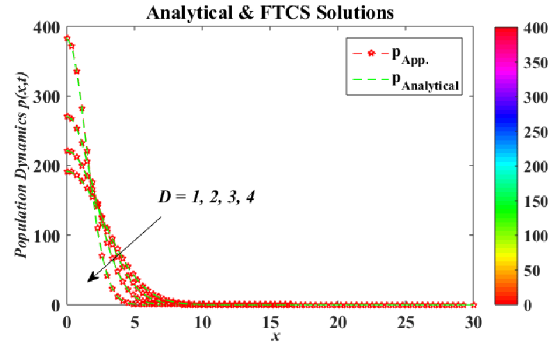
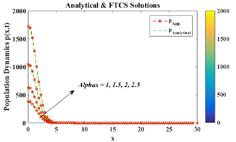
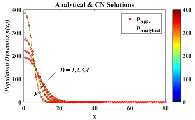
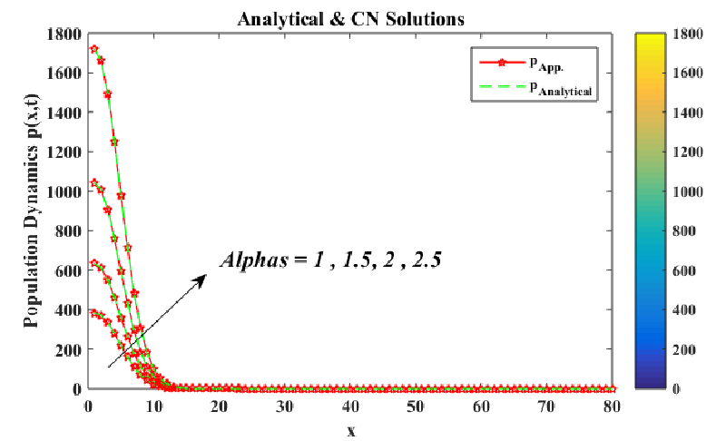
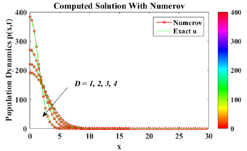
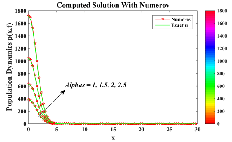
Figure 1 shows the results produced by crank Nicolson. A comparison is also provided for the detailed analysis. The parameter α is taken as constant and parameter D is varied. It’s obvious from the plot that as soon as we increase the dispersion rate D, the area occupied by the population shows an upsurge which is quite a depiction of the physical phenomenon called dispersion. Figure 2 shows the results produced by the same scheme as in Figure 1. Here the plots are drawn using D as constant and variation is taken in parameter α. The increased values of α present an interesting phenomenon. As we enhance the values of alpha, the population starts increasing which is very easy to judge. Figure 3 shows the results produced by the FTCS scheme. Here dispersion rate is taken fixed and α is increased uniformly. The results are quite obvious and cause a significant increase in the population. Figure 4 is showing the comparison between analytical and FTCS schemes. The parameter D is changed keeping alpha fixed. Figures 5,6 show the plots taken by Numerov’s method using the same technique as previously done.

Tables 1-3 display the results as obtained through simulations performed by employing numerical techniques such as Numerov’s method, FTCS and Crank Nicolson schemes respectively, A comparison between the analytical and approximated results is made by calculating the relative error. The results show the efficiency of the schemes. By comparing the results of numerical techniques, we found that the percentage error of the Crank-Nicolson scheme is less than the other two schemes.

Discussion

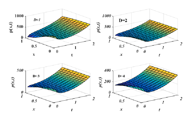
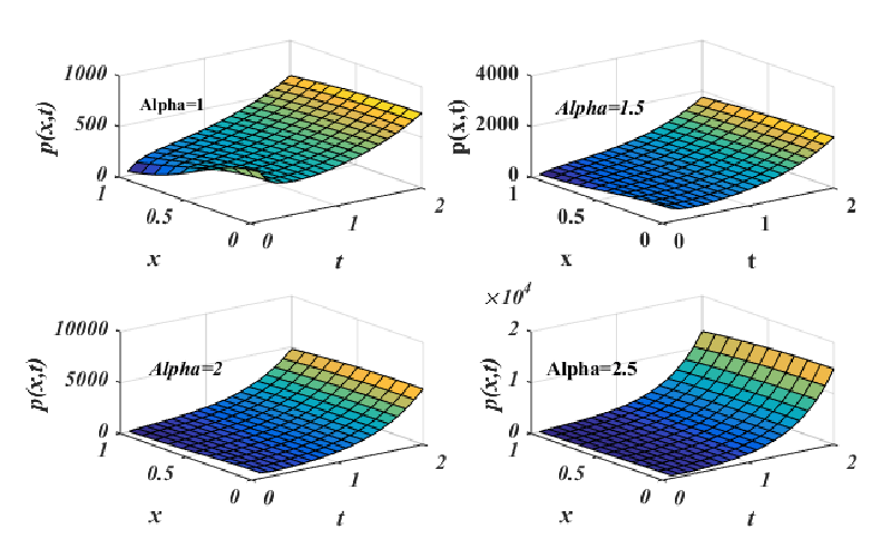
While making the simulation we kept some parameters unchanged and the rest of those were allowed to vary to show our obtained results graphically. For validation of their efficiency, we gradually made a comparison with the analytical solution. Figures 1,2 depicts the efficiency of the FTCS scheme whereas Figures 3,4 give a comparison between the Crank Nicolson scheme and exact solution. Figures 5,6 indicate the results of Numerov’s method and comparison with the exact solution as well. Figures 7(a-d), 8(a-d) are reflecting the results of surface plots of the exact solution whereas in Figure 7 dispersion was allowed to vary and the growth rate was kept constant and in Figure 8 its reverse was applied [30-32].

Conclusion

The linear model carrying the diffusion factor was adopted to analyze the population dispersion model in which the population was initially stagnant at a single point. This model revolves around a wonderful combination of dispersion and growth rates. Schemes applied during simulation proved surprisingly efficient. The numerical computation leads us to the result that when we find the average error produced by the schemes applied, the average error of the Crank Nicolson scheme is much less as compared to the other schemes. The Crank Nicolson is more efficient for the current population dispersion model. Plots indicate that the rise of the growth rate graph moves up vertically and with the rise of dispersion rate it initially moves forward and after a brief period it starts grazing along with the earth or horizontal line. Moreover, it resonates with the general concept of population growth. In the recent future, we are aimed at incorporating birth and death rates along with growth and dispersion and will make a comparison of the results of both.

1. Gray BF, Kirwan NA. Growth rates of yeast colonies on solid media. Biophys Chem. 1974 Feb;1(3):204-13. doi: 10.1016/0301-4622(74)80006-2. PMID: 4609508.
2. Chen SC. Effect of habitat fragmentation on seed dispersal ability of a wind-dispersed annual in an agroecosystem. Agriculture. Ecol Evol. 2020; 304: 107138.
3. James F, Mansur ET, Sacerdote B. Geographic dispersion of economic shocks: Evidence from the fracking revolution. Am Econ Rev. 2017; 107: 1313-1334.
4. Macfarlan SJ, Schacht R, Schniter E, Garcia JJ, Guevara Beltran D, Lerback J. The role of dispersal and school attendance on reproductive dynamics in small, dispersed populations: Choyeros of Baja California Sur, Mexico. PLoS One. 2020 Oct 7;15(10):e0239523. doi: 10.1371/journal.pone.0239523. PMID: 33027256; PMCID: PMC7540897.
5. Shoemaker LG, Sullivan LL, Donohue I, Cabral JS, Williams RJ, Mayfield MM, Chase JM, Chu C, Harpole WS, Huth A, HilleRisLambers J, James ARM, Kraft NJB, May F, Muthukrishnan R, Satterlee S, Taubert F, Wang X, Wiegand T, Yang Q, Abbott KC. Integrating the underlying structure of stochasticity into community ecology. Ecology. 2020 Feb;101(2):e02922. doi: 10.1002/ecy.2922. Epub 2019 Dec 26. PMID: 31652337; PMCID: PMC7027466.
6. Soares J, Fernandes R, Brito D, Oliveira H, Neuparth T, Martins I, Santos MM. Environmental risk assessment of accidental marine spills: A new approach combining an online dynamic Hazardous and Noxious substances database with numerical dispersion, risk and population modelling. Sci Total Environ. 2020 May 1;715:136801. doi: 10.1016/j.scitotenv.2020.136801. Epub 2020 Jan 18. PMID: 32007875.
7. Koki T, Tokuda M. Negative correlation between dispersal investment and canopy openness among populations of the ant-dispersed sedge, Carex lanceolata. Plant Ecol. 2020; 221: 1105-1115.
8. Israel G. The emergence of biomathematics and the case of population dynamics: a revival of mechanical reductionism and Darwinism. Sci Context. 1993 Autumn;6(2):469-509. doi: 10.1017/s0269889700001484. PMID: 11623401.
9. Shaher M, Qaralleh R. Numerical approximations and Padé approximants for a fractional population growth model. Appl Math Model. 2007; 31: 1907-1914.
10. Ismail HNA, Kamal RR, Ghada SES. Solitary wave solutions for the general KDV equation by Adomian decomposition method. Appl Math Comput. 2004; 154: 17-29.
11. Segel LA. Mathematical models in biology (Leah Edelstein-Keshet). 1988; 679.
12. Seng VKA, Cherruault Y. Adomian's polynomials for nonlinear operators. Math Comput Model. 1996; 24: 59-65.
13. Yves C. Convergence of Adomian's method. Kybernetes. 1989; 18: 31-38.
14. Rèpaci A. Nonlinear dynamical systems: on the accuracy of Adomian's decomposition method. Appl Math Lett. 1990; 3: 35-39.
15. Cherruault Y, Adomian G. Decomposition methods: a new proof of convergence. Math Comput Model. 1993; 18: 103-106.
16. Ames WF. Numerical methods for partial differential equations. Academic Press, 2014.
17. Adomaitis RA, Yi-hung L, Hsiao-Yung C. A computational framework for boundary-value problem-based simulations. Simulation. 2000; 74: 28-38.
18. Hasnain S, Muhammad S, Daoud SM. Two-Dimensional nonlinear reaction-diffusion equation with time efficient scheme. Am J Comput Math. 2017; 7: 183-194.
19. Hasnain S, Muhammad S. Numerical study of one-dimensional Fishers KPP equation with finite difference schemes. Am J Comput Math. 2017; 7: 70-83.
20. Abushaikha AS, Kirill MT. A fully implicit mimetic finite difference scheme for general purpose subsurface reservoir simulation with full tensor permeability. J Comput Phys. 2020; 406: 109194.
21. Xu D, Wenlin Q, Jing G. A compact finite difference scheme for the fourth‐order time‐fractional integro‐differential equation with a weakly singular kernel. Numer Methods Partial Differ Equ. 2020; 36: 439-458.
22. Safdari H. Convergence analysis of the space fractional-order diffusion equation based on the compact finite difference scheme. Comput Appl Math. 2020; 39: 1-15.
23. Saqib M, Shahid H, Daoud SM. Computational solutions of two-dimensional convection-diffusion equation using crank-nicolson and time efficient ADI. Am J Comput Math. 2017; 7: 208-227.
24. Li Z, Kazufumi I. The immersed interface method: numerical solutions of PDEs involving interfaces and irregular domains. Soc Indust Appl Math. 2006.
25. Hasnain S. Efficiency of numerical schemes for two dimensional Gray Scott model. AIP Advances. 2019; 9.
26. Hasnain S, Muhammad S, Nawaf AH. Finite Difference Implicit Schemes to Coupled Two-Dimension Reaction-Diffusion System. J Appl Math Phy. 2018; 6: 737-753.
27. Xue G, Yunjie G, Hui F. The splitting Crank–Nicolson scheme with intrinsic parallelism for solving parabolic equations. J Funct Space. 2020; 1-12.
28. Gan X, Dengguo X. On the convergence of a crank–nicolson fitted finite volume method for pricing American bond options. Math Probl Eng. 2020; 2020: 1-13.
29. Luo Z, Wenrui J. The Crank–Nicolson finite spectral element method and numerical simulations for 2D non‐stationary Navier–Stokes equations. Math Methods Appl Sci. 2020; 43: 2276-2288.
30. Hasnain S, Muhammad S, Daoud SM. Fourth-order Douglas implicit scheme for solving three dimensions reaction-diffusion equation with non-linear source term. AIP Advances. 2017; 7.
31. Craig IJD, Sneyd AD. An alternating-direction implicit scheme for parabolic equations with mixed derivatives. Comput Math Applicat. 1988; 16: 341-350.
32. Steidl G, Tanja T. Removing multiplicative noise by Douglas-Rachford splitting methods. J Math Imaging Vis. 2010; 36: 168-184.
33. Stinson DR, Reto S. Provably secure distributed Schnorr signatures and a (t, n) threshold scheme for implicit certificates. Australasian Conference on Information Security and Privacy. Berlin, Heidelberg: Springer Berlin Heidelberg, 2001.
34. Ixaru LGR, Rizea M. Numerov method maximally adapted to the schr6dinger equation. J Comput Phy. 1987; 73: 306-324.
35. Alexander Z. The Numerov-Crank-Nicolson scheme on a non-uniform mesh for the time-dependent Schrödinger equation on the half-axis. Kin Relat Model. 2015; 8: 587-613.
36. Zlotnik A, Alla R. On a Numerov–Crank–Nicolson–Strang scheme with discrete transparent boundary conditions for the Schrödinger equation on a semi-infinite strip. Appl Num Math. 2015; 93: 279-294.
37. Babuska IB. Numerical Stability in Mathematical Analysis. IFIP Congress. North-Holland, Amsterdam. 1968; 11: 23.
38. Roache PJ. Computational fluid dynamics (Book- Computational fluid dynamics.). Albuquerque, N. Mex., Hermosa Publishers. 1972; 437.
39. Saqib M, Muhammad FA, Iqtadar H. Numerical study to coupled three-dimensional reaction-diffusion system. IEEE Access. 2019; 7: 46695-46705.
40. Çelik E, Durmuş A. Nonlinear regression applications in modeling over-dispersion of bird populations. J Anim Plant Sci. 2020; 30: 345-354.