Numerical simulations in a generalized Liénard's type system

In this note we present some numerical simulations of the asymptotic behavior of a Generalized Liénard Equation, taking into account a recently defined differential operator. We must point out that these numerical variations have not been obtained as usual: by varying the functions of the right member of the system considered, but, on the contrary, by varying the kernels and the order of the generalized operator used. The above provides breadth and generality to the results obtained, which complement some known in the literature.

Introduction

The classical method of Lyapunov for studying stability and asymptotic stability is based on a suitable function satisfying some properties (called Lyapunov's Functions). This method, usually named the Second Method, originated in the fundamental memoir of the Russian mathematician Alexander Mijailovich Lyapunov, published in Russian in 1892, translated into French in 1907 (reprinted in the forty) and in English years later, see [1]. Since that time this area has been extensively (perhaps even exhaustively) investigated. Statements and proofs of mathematical results underlying the method and numerous examples and references can be found in the books [2-7] and the bibliography listed therein.

The Liénard Equation, one of the icons of Nonlinear Analysis, is a second-order nonlinear differential equation that appears in various areas of physics and engineering. Its importance lies in several aspects:

Nonlinear oscillations

The Liénard Equation describes nonlinear systems that exhibit damped and forced oscillations. This is crucial to understand and model phenomena in which linearity is not sufficient to represent the behavior of the system.

Study of non-conservative systems

The equation is useful for studying non-conservative systems, where energy is not conserved. This is common in systems that experience friction, drag, or other dissipative forces.

Chaos theory

The Liénard Equation can show chaotic behavior, meaning that the solutions are highly sensitive to initial conditions. The study of chaotic systems is crucial in chaos theory and has applications in the prediction of certain natural phenomena.

Stability analysis

The equation is used in the stability analysis of nonlinear dynamic systems. The study of stability is essential to ensure that a system responds predictably to perturbations and changes in initial conditions.

Control engineering

In the design of nonlinear control systems, the Liénard Equation is relevant to understanding and predicting the behavior of physical systems. This is crucial in engineering applications, such as industrial process control and electromechanical systems.

Mathematical research

The equation has been the object of study in mathematical research, contributing to the development of methods and techniques to solve nonlinear differential equations. This has broader implications in the field of differential equation theory and dynamical systems.

In summary, the Liénard Equation plays a key role in the understanding of non-linear, chaotic, and non-conservative systems in various scientific and engineering disciplines. Its study has led to the development of analytical and numerical tools that are fundamental for the understanding and design of complex and dynamic systems. Hence, research aimed at the qualitative study of Liénard-type system solutions has an impact not only from a theoretical point of view but also in applications.

On the other hand, the problem of continuability of solutions is of paramount importance in the study of qualitative properties. For example, in [8] some properties of the system

$\{\begin{array}{ll}\dot{x}\mathrm{<mo>=</mo>}\alpha \mathrm{<mo\; stretchy="false">(</mo>}y\mathrm{<mo\; stretchy="false">)</mo>}-\beta \mathrm{<mo\; stretchy="false">(</mo>}y\mathrm{<mo\; stretchy="false">)</mo>}F\mathrm{<mo\; stretchy="false">(</mo>}x\mathrm{<mo\; stretchy="false">)</mo>,}\hfill & \hfill \\ \dot{y}\mathrm{<mo>=</mo>}-g\mathrm{<mo\; stretchy="false">(</mo>}x\mathrm{<mo\; stretchy="false">)</mo>,}\hfill & \hfill \end{array}\text{ (1)}$

was studied under suitable assumptions. A particular case of the above system is the well-known Liénard equation

$\ddot{x}+f\mathrm{<mo\; stretchy="false">(</mo>}x\mathrm{<mo\; stretchy="false">)</mo>}\dot{x}+g\mathrm{<mo\; stretchy="false">(</mo>}x\mathrm{<mo\; stretchy="false">)</mo><mo>=</mo>0,}\text{ (2)}$

Where f(x), g(x) are continuous functions and g(0) =0, are the subject of detailed studies by various authors due to many applications in a variety of domains in science and technology, see for example [9-16] and classical sources [17-19].

Let $F\mathrm{<mo\; stretchy="false">(</mo>}x\mathrm{<mo\; stretchy="false">)</mo><mo>=</mo>}{\displaystyle {\int }_0^x}f\mathrm{<mo\; stretchy="false">(</mo>}s\mathrm{<mo\; stretchy="false">)</mo>}ds$ we obtain an equivalent system to equation (2):

$\{\begin{array}{ll}\dot{x}\mathrm{<mo>=</mo>}y-F\mathrm{<mo\; stretchy="false">(</mo>}x\mathrm{<mo\; stretchy="false">)</mo>,}\hfill & \hfill \\ \dot{y}\mathrm{<mo>=</mo>}-g\mathrm{<mo\; stretchy="false">(</mo>}x\mathrm{<mo\; stretchy="false">)</mo>,}\hfill & \hfill \end{array}\text{ (3)}$

Fractional calculus studies problems with derivatives and integrals of real or complex order. As a purely mathematical field, the theory of fractional calculus was brought up for the first time in the XVIIth century and since then many renowned scientists worked on this topic, among them Euler, Laplace, Fourier, Abel, Liouville, and Riemann (see [20]). Today there is a vast literature on this subject, and many works and researchers multiply day by day in the world showing the most varied applications. The most common applications are currently found in Rheology, Quantum Biology, Electrochemistry, Dispersion Theory, Diffusion, Transport Theory, Probability and Statistics, Potential Theory, Elasticity, Viscosity, Automatic Control Theory, .

After presenting the fractional integrals it is possible to define the fractional derivatives associated with these operators. Fractional derivatives and fractional integrals are extensions of ordinary calculus, by considering derivatives of arbitrary real or complex order, and a general form for multiple integrals. Although mathematicians have wondered since the very beginning of calculus about these questions, only recently they have proven their usefulness and since then important results have appeared not only in mathematics but also in physics, applied engineering, biology, etc. One question that is important is what type of fractional operator should be considered since we have in hand several distinct definitions and the choice depends on the considered problem.

In the literature many different types of fractional operators have been proposed, here, we show that various of that different notions of derivatives, can be considered particular cases of our definition and, even more relevant, that it is possible to establish a direct relationship between global (classical) and local derivatives, the latter not very accepted by the mathematical community, under two arguments: their local character and compliance with the Leibniz Rule. To facilitate the understanding of the scope of our definition, we present the best-known definitions of integral operators and their corresponding differential operators (for more details you can consult [21]). Without many difficulties, we can extend these definitions, for any higher order.

A general integral operator

In [22] was presented an integral operator generalized, which contains in particular cases, many of the well-known integral operators, both integer order and not. First, we will present the definition of the generalized derivative, see [23] (see also [24] and [25]) which was defined in the following way.

Definition 1: Given a function $f\mathrm{<mo>:</mo><mo\; stretchy="false">[</mo>0,}+\infty \mathrm{<mo\; stretchy="false">)</mo>}\to ℝ$ . Then the N-derivative of f of order α is defined by

$N_F^{\alpha }f\mathrm{<mo\; stretchy="false">(</mo>}t\mathrm{<mo\; stretchy="false">)</mo><mo>=</mo>}\underset{\epsilon \to 0}{\lim }\frac{f\mathrm{<mo\; stretchy="false">(</mo>}t+\epsilon F\mathrm{<mo\; stretchy="false">(</mo>}t\mathrm{,}\alpha \mathrm{<mo\; stretchy="false">)</mo><mo\; stretchy="false">)</mo>}-f\mathrm{<mo\; stretchy="false">(</mo>}t\mathrm{<mo\; stretchy="false">)</mo>}}{\epsilon }\text{ (4)}$

for all t0, α∈(0,1) being F(α,t) is some function. If f is α - differentiable in some (0,), and $\underset{t\to 0^{+}}{\lim }{N}_F^{\alpha }f\mathrm{<mo\; stretchy="false">(</mo>}t\mathrm{<mo\; stretchy="false">)</mo>}$ exists, then define $N_F^{\alpha }f\mathrm{<mo\; stretchy="false">(</mo>0<mo\; stretchy="false">)</mo><mo>=</mo>}\underset{t\to 0^{+}}{\lim }{N}_F^{\alpha }f\mathrm{<mo\; stretchy="false">(</mo>}t\mathrm{<mo\; stretchy="false">)</mo>}$ , note that if f is differentiable, then $N_F^{\alpha }f\mathrm{<mo\; stretchy="false">(</mo>}t\mathrm{<mo\; stretchy="false">)</mo><mo>=</mo>}F\mathrm{<mo\; stretchy="false">(</mo>}t\mathrm{,}\alpha \mathrm{<mo\; stretchy="false">)</mo>}{f}^{\prime }\mathrm{<mo\; stretchy="false">(</mo>}t\mathrm{<mo\; stretchy="false">)</mo>}$ where $f^{\prime }\mathrm{<mo\; stretchy="false">(</mo>}t\mathrm{<mo\; stretchy="false">)</mo>}$ is the ordinary derivative.

Some particular cases of this operator are the following:

I) F(x,α) ≡ 1, in this case, we have the ordinary derivative.

II) $F\mathrm{<mo\; stretchy="false">(</mo>}x\mathrm{,}\alpha \mathrm{<mo\; stretchy="false">)</mo><mo>=</mo>}{e}^{x^{-\alpha }}$ . In this case we obtain, from Definition 1, the non-conformable derivative $N_1^{\alpha }f\mathrm{<mo\; stretchy="false">(</mo>}x\mathrm{<mo\; stretchy="false">)</mo>}$ defined in [26] (see also [27]).

III) F(x,α) → e^(1-α)x, this kernel satisfies that F(x,α) → 1 as α → 1, a conformable derivative used in [28].

IV) F(x,α) → x^1-α with this kernel we have F(x,α) → 0 as α → 1 (see [29]), a conformable derivative.

V) F(x,α) → x^α with this kernel we have F(x,α) → x as α → 1 (see 30]). It is clear that since it is a non-conformable derivative, the results will differ from those obtained previously, which enhances the study of these cases.

VI) F(x,α) → x^-α with this kernel we have F(x,α) → x^-1 as α → 1 This is the derivative studied in [31]. As in the previous case, the results obtained have not been reported in the literature.

Now, we give the definition of a general fractional integral. Throughout the work, we will consider that the integral operator kernel T defined below is an absolutely continuous function.

Definition 2: Let I be an interval $I\subseteq ℝ\text{, }a\mathrm{,}t\in Iand\alpha \in ℝ$ . The integral operator $J_{T\mathrm{,}a}^{\alpha }$ , is defined for every locally integrable function f on I as

$J_{T\mathrm{,}a}^{\alpha }\mathrm{<mo\; stretchy="false">(</mo>}f\mathrm{<mo\; stretchy="false">)</mo><mo\; stretchy="false">(</mo>}b\mathrm{<mo\; stretchy="false">)</mo><mo>=</mo>}{\displaystyle {\int }_a^b}\frac{f\mathrm{<mo\; stretchy="false">(</mo>}t\mathrm{<mo\; stretchy="false">)</mo>}}{T\left(t\mathrm{,}\alpha \right)}dt\mathrm{.}\text{ (5)}$

Remark 3: It is easy to see that the case of the $J_T^{\alpha }$ operator defined above contains, as particular cases, the integral operators obtained from conformable and non-conformable local derivatives, Interested readers can consult [22].

The following results are generalizations of the known results of the integer order Calculus.

Proposition 4: Let I be an interval $I\subseteq ℝ\text{,}a\in I,\mathrm{0<mo><</mo>}\alpha \le 1$ and f a $\alpha$ -differentiable function on I such that $f^{\prime }$ is a locally integrable function on I. Then, we have for all x∈I

$J_{T\mathrm{,}a+}^{\alpha }\mathrm{<mo\; stretchy="false">(</mo>}{N}_T^{\alpha }\mathrm{<mo\; stretchy="false">(</mo>}f\mathrm{<mo\; stretchy="false">)</mo><mo\; stretchy="false">)</mo><mo\; stretchy="false">(</mo>}x\mathrm{<mo\; stretchy="false">)</mo><mo>=</mo>}f\mathrm{<mo\; stretchy="false">(</mo>}x\mathrm{<mo\; stretchy="false">)</mo>}-f\mathrm{<mo\; stretchy="false">(</mo>}a\mathrm{<mo\; stretchy="false">)</mo>.}$

Proposition 5: Let I be an interval $I\subseteq ℝ\text{,}a\in Iand\alpha \in \mathrm{<mo\; stretchy="false">(</mo>0,1<mo\; stretchy="false">]</mo>}$ .

$N_T^{\alpha }\mathrm{<mo\; stretchy="false">(</mo>}{J}_{T\mathrm{,}a+}^{\alpha }\mathrm{<mo\; stretchy="false">(</mo>}f\mathrm{<mo\; stretchy="false">)</mo><mo\; stretchy="false">)</mo><mo\; stretchy="false">(</mo>}x\mathrm{<mo\; stretchy="false">)</mo><mo>=</mo>}f\mathrm{<mo\; stretchy="false">(</mo>}x\mathrm{<mo\; stretchy="false">)</mo>,}$

for every continuous function f on I and a,t∈I.

In [29] it is defined the integral operator $J_{F\mathrm{,}a}^{\alpha }$ for the choice of the function F given by $F\mathrm{<mo\; stretchy="false">(</mo>}x\mathrm{,}\alpha \mathrm{<mo\; stretchy="false">)</mo><mo>=</mo>}{x}^{1-\alpha }$ , and [29, Theorem 3.1] shows

$N^{\alpha }{J}_{x^{1-\alpha }\text{}\mathrm{,}a}^{\alpha }\mathrm{<mo\; stretchy="false">(</mo>}f\mathrm{<mo\; stretchy="false">)</mo><mo\; stretchy="false">(</mo>}x\mathrm{<mo\; stretchy="false">)</mo><mo>=</mo>}f\mathrm{<mo\; stretchy="false">(</mo>}x\mathrm{<mo\; stretchy="false">)</mo>,}$

for every continuous function f on I, a, x∈I and α∈(0,1]. Hence, Proposition 5 extends to any T of this important equality.

Theorem 6: Let I be an interval $I\subseteq ℝ\text{,}a,b\in Iand\alpha \in ℝ$ . Suppose that f,g are locally integrable functions on I, and $k_1\mathrm{,}{k}_2\in ℝ$ . Then we have

(1) $J_{T\mathrm{,}a}^{\alpha }\mathrm{<mo\; stretchy="false">(</mo>}{k}_{1}f+k_{2}g\mathrm{<mo\; stretchy="false">)</mo><mo\; stretchy="false">(</mo>}x\mathrm{<mo\; stretchy="false">)</mo><mo>=</mo>}{k}_1{J}_{T\mathrm{,}a}^{\alpha }f\mathrm{<mo\; stretchy="false">(</mo>}x\mathrm{<mo\; stretchy="false">)</mo>}+k_2{J}_{T\mathrm{,}a}^{\alpha }g\mathrm{<mo\; stretchy="false">(</mo>}x\mathrm{<mo\; stretchy="false">)</mo>,}$

(2) if $f\ge g$ , then $J_{T\mathrm{,}a}^{\alpha }f\mathrm{<mo\; stretchy="false">(</mo>}x\mathrm{<mo\; stretchy="false">)</mo>}\ge J_{T\mathrm{,}a}^{\alpha }g\mathrm{<mo\; stretchy="false">(</mo>}x\mathrm{<mo\; stretchy="false">)</mo>}$ for every t∈I with t≥a,

(3) $\left|J_{T\mathrm{,}a}^{\alpha }f\mathrm{<mo\; stretchy="false">(</mo>}x\mathrm{<mo\; stretchy="false">)</mo>}\right|\le J_{T\mathrm{,}a}^{\alpha }\left|f\right|\mathrm{<mo\; stretchy="false">(</mo>}x\mathrm{<mo\; stretchy="false">)</mo>}$ for every t∈I with t≥a,

(4) ${\displaystyle {\int }_a^b}\frac{f\mathrm{<mo\; stretchy="false">(</mo>}s\mathrm{<mo\; stretchy="false">)</mo>}}{T\mathrm{<mo\; stretchy="false">(</mo>}s\mathrm{,}\alpha \mathrm{<mo\; stretchy="false">)</mo>}}ds\mathrm{<mo>=</mo>}{J}_{T\mathrm{,}a}^{\alpha }f\mathrm{<mo\; stretchy="false">(</mo>}x\mathrm{<mo\; stretchy="false">)</mo>}-J_{T\mathrm{,}b}^{\alpha }f\mathrm{<mo\; stretchy="false">(</mo>}x\mathrm{<mo\; stretchy="false">)</mo><mo>=</mo>}{J}_{T\mathrm{,}a}^{\alpha }f\mathrm{<mo\; stretchy="false">(</mo>}x\mathrm{<mo\; stretchy="false">)</mo><mo\; stretchy="false">(</mo>}b\mathrm{<mo\; stretchy="false">)</mo>}$ for every t∈I.

Let $C^1\mathrm{<mo\; stretchy="false">[</mo>}a\mathrm{,}b\mathrm{<mo\; stretchy="false">]</mo>}$ be the set of functions f with first ordinary derivative continuous on [a,b], we consider the following norms on :

${\Vert F\Vert }_C\mathrm{<mo>=</mo>}\underset{\mathrm{<mo\; stretchy="false">[</mo>}a\mathrm{,}b\mathrm{<mo\; stretchy="false">]</mo>}}{{\displaystyle \max }}\left|f\mathrm{<mo\; stretchy="false">(</mo>}x\mathrm{<mo\; stretchy="false">)</mo>}\right|\mathrm{,}{\Vert F\Vert }_{C^1}\mathrm{<mo>=</mo>}\left\{\underset{\mathrm{<mo\; stretchy="false">[</mo>}a\mathrm{,}b\mathrm{<mo\; stretchy="false">]</mo>}}{{\displaystyle \max }}\left|f\mathrm{<mo\; stretchy="false">(</mo>}x\mathrm{<mo\; stretchy="false">)</mo>}\right|+\underset{\mathrm{<mo\; stretchy="false">[</mo>}a\mathrm{,}b\mathrm{<mo\; stretchy="false">]</mo>}}{{\displaystyle \max }}\left|f^{\prime }\mathrm{<mo\; stretchy="false">(</mo>}x\mathrm{<mo\; stretchy="false">)</mo>}\right|\right\}$

Theorem 7: The fractional derivatives $N_{T\mathrm{,}a+}^{\alpha }f\mathrm{<mo\; stretchy="false">(</mo>}x\mathrm{<mo\; stretchy="false">)</mo>}and{N}_{T\mathrm{,}b-}^{\alpha }f\mathrm{<mo\; stretchy="false">(</mo>}x\mathrm{<mo\; stretchy="false">)</mo>}$ are bounded operators from $C^1\mathrm{<mo\; stretchy="false">[</mo>}a\mathrm{,}b\mathrm{<mo\; stretchy="false">]</mo>}toC\mathrm{<mo\; stretchy="false">[</mo>}a\mathrm{,}b\mathrm{<mo\; stretchy="false">]</mo>}$ with

$\left|N_{T\mathrm{,}a+}^{\alpha }f\mathrm{<mo\; stretchy="false">(</mo>}x\mathrm{<mo\; stretchy="false">)</mo>}\right|\le K{\Vert F\Vert }_C{\Vert f\Vert }_{C^1}\mathrm{,}\text{ (6)}$

$\left|N_{T\mathrm{,}b-}^{\alpha }f\mathrm{<mo\; stretchy="false">(</mo>}x\mathrm{<mo\; stretchy="false">)</mo>}\right|\le K{\Vert F\Vert }_C{\Vert f\Vert }_{C^1}\mathrm{,}\text{ (7)}$

where the constant K, may be dependent on the derivative frame considered.

Remark 8: From previous results we obtain that the derivatives $N_{T\mathrm{,}a+}^{\alpha }f\mathrm{<mo\; stretchy="false">(</mo>}x\mathrm{<mo\; stretchy="false">)</mo>}and{N}_{T\mathrm{,}b-}^{\alpha }f\mathrm{<mo\; stretchy="false">(</mo>}x\mathrm{<mo\; stretchy="false">)</mo>}$ are well defined.

Theorem 9: (Integration by parts) Let $f\mathrm{,}g\mathrm{<mo>:</mo><mo\; stretchy="false">[</mo>}a\mathrm{,}b\mathrm{<mo\; stretchy="false">]</mo>}\to ℝ$ differentiable functions and α∈(0,1]. Then, the following property hold

$J_{T\mathrm{,}a+}^{\alpha }\mathrm{<mo\; stretchy="false">(</mo><mo\; stretchy="false">(</mo>}f\mathrm{<mo\; stretchy="false">)</mo><mo\; stretchy="false">(</mo>}{N}_{T\mathrm{,}a+}^{\alpha }g\mathrm{<mo\; stretchy="false">(</mo>}x\mathrm{<mo\; stretchy="false">)</mo><mo\; stretchy="false">)</mo><mo\; stretchy="false">)</mo><mo>=</mo>}{\left[f\mathrm{<mo\; stretchy="false">(</mo>}x\mathrm{<mo\; stretchy="false">)</mo>}g\mathrm{<mo\; stretchy="false">(</mo>}x\mathrm{<mo\; stretchy="false">)</mo>}\right]}_a^b-J_{T\mathrm{,}a+}^{\alpha }\mathrm{<mo\; stretchy="false">(</mo><mo\; stretchy="false">(</mo>}g\mathrm{<mo\; stretchy="false">)</mo><mo\; stretchy="false">(</mo>}{N}_{T\mathrm{,}a+}^{\alpha }f\mathrm{<mo\; stretchy="false">(</mo>}x\mathrm{<mo\; stretchy="false">)</mo><mo\; stretchy="false">)</mo><mo\; stretchy="false">)</mo>.}\text{ (8)}$

In [32] the following system was studied:

$\begin{array}{l}{N}_T^{\gamma }x\mathrm{<mo>=</mo>}E\mathrm{<mo\; stretchy="false">(</mo>}x\mathrm{,}y\mathrm{<mo\; stretchy="false">)</mo>}\hfill \\ N_T^{\gamma }y\mathrm{<mo>=</mo>}-p\mathrm{<mo\; stretchy="false">(</mo>}y\mathrm{<mo\; stretchy="false">)</mo>}g\mathrm{<mo\; stretchy="false">(</mo>}x\mathrm{<mo\; stretchy="false">)</mo>}\hfill \end{array}\}\text{, (9)}$

where $E\mathrm{<mo\; stretchy="false">(</mo>}x\mathrm{,}y\mathrm{<mo\; stretchy="false">)</mo><mo>=</mo>}a\mathrm{<mo\; stretchy="false">(</mo>}x\mathrm{,}y\mathrm{<mo\; stretchy="false">)</mo>}H\mathrm{<mo\; stretchy="false">(</mo>}x\mathrm{,}y\mathrm{<mo\; stretchy="false">)</mo>}\text{ with }H\mathrm{<mo\; stretchy="false">(</mo>}x\mathrm{,}y\mathrm{<mo\; stretchy="false">)</mo><mo>=</mo>}H\mathrm{<mo\; stretchy="false">(</mo>}\alpha \mathrm{<mo\; stretchy="false">(</mo>}y\mathrm{<mo\; stretchy="false">)</mo>}-\beta \mathrm{<mo\; stretchy="false">(</mo>}y\mathrm{<mo\; stretchy="false">)</mo>}F\mathrm{<mo\; stretchy="false">(</mo>}x\mathrm{<mo\; stretchy="false">)</mo><mo\; stretchy="false">)</mo>}$ while the functions in above system are continuous real functions in their arguments.

Throughout this paper we will use the following notations (F(x) as above and E_a,p is the bipárametric Mittag-Leffler function):

$G\mathrm{<mo\; stretchy="false">(</mo>}x\mathrm{<mo\; stretchy="false">)</mo><mo>=</mo>}{\displaystyle {\int }_0^x}g\mathrm{<mo\; stretchy="false">(</mo>}s\mathrm{<mo\; stretchy="false">)</mo>}ds\mathrm{,}{E}_{a\mathrm{,}p}^{\alpha }\mathrm{<mo\; stretchy="false">(</mo>}y\mathrm{<mo\; stretchy="false">)</mo><mo>=</mo>}{E}_{a\mathrm{,}p}^{\alpha }\mathrm{<mo\; stretchy="false">(</mo>0,}y\mathrm{<mo\; stretchy="false">)</mo><mo>=</mo>}{\displaystyle {\int }_0^y}\frac{a\mathrm{<mo\; stretchy="false">(</mo>0,}s\mathrm{<mo\; stretchy="false">)</mo>}H\mathrm{<mo\; stretchy="false">(</mo>}\alpha \mathrm{<mo\; stretchy="false">(</mo>}s\mathrm{<mo\; stretchy="false">)</mo><mo\; stretchy="false">)</mo>}}{p\mathrm{<mo\; stretchy="false">(</mo>}s\mathrm{<mo\; stretchy="false">)</mo>}}ds\mathrm{.}$

Our objective is to illustrate that in the system (9), under different local operators, the examples and counterexamples known from the literature continue to hold. Obviously, our conclusions cover the systems (1) and (3), and therefore, for the equation (2).

Results

The following results are useful in the subsequence ([32]).

Theorem 10: Under the following assumptions:

i) E(x,y) is a differentiable function with

$\underset{R^2}{\sup }\frac{\partial E}{\partial x}\mathrm{<mo\; stretchy="false">(</mo>}x\mathrm{,}y\mathrm{<mo\; stretchy="false">)</mo><mo><</mo>}+\infty$

and

$\underset{y\to \pm \infty }{\lim \sup }{E}_{a\mathrm{,}p}^{\alpha }\mathrm{<mo\; stretchy="false">(</mo>}y\mathrm{<mo\; stretchy="false">)</mo><mo>=</mo>}\pm \infty \mathrm{.}$

ii) p(y)>0 for all $y\in ℝ$ .

iii) There exists a positive constant λ such that $g\mathrm{<mo\; stretchy="false">(</mo>}x\mathrm{<mo\; stretchy="false">)</mo>}F\mathrm{<mo\; stretchy="false">(</mo>}x\mathrm{<mo\; stretchy="false">)</mo>}\ge -\lambda$ , ${\displaystyle {\int }_0^t}x\mathrm{<mo\; stretchy="false">(</mo>}s\mathrm{<mo\; stretchy="false">)</mo>}g\mathrm{<mo\; stretchy="false">(</mo>}x\mathrm{<mo\; stretchy="false">(</mo>}s\mathrm{<mo\; stretchy="false">)</mo><mo\; stretchy="false">)</mo>}ds\ge -\lambda$ for all $x\in ℝ$ and $\underset{x\in R}{\left|F\mathrm{<mo\; stretchy="false">(</mo>}x\mathrm{<mo\; stretchy="false">)</mo>}\right|}\mathrm{<mo><</mo>}+\infty$ .

iv) $a\in C^{\mathrm{1,0}}\mathrm{<mo\; stretchy="false">(</mo>}{ℝ}^2\mathrm{<mo\; stretchy="false">)</mo>}$ such that $a\mathrm{<mo\; stretchy="false">(</mo>}x\mathrm{,}y\mathrm{<mo\; stretchy="false">)</mo><mo>></mo>0}$ for all x and y, and $\underset{x\to \pm \infty }{\lim \sup }a\mathrm{<mo\; stretchy="false">(</mo>}x\mathrm{,}y\mathrm{<mo\; stretchy="false">)</mo><mo><</mo>}+\infty$ for all y.

then all solutions of system (9) can be defined for all t.

Theorem 11: In addition to i) and iv) suppose that the following assumptions are satisfied:

ii*) $p\mathrm{<mo\; stretchy="false">(</mo>}y\mathrm{<mo\; stretchy="false">)</mo><mo>></mo>0}$ for all $y\in ℝ$ , $P\mathrm{<mo\; stretchy="false">(</mo>}\pm \infty \mathrm{<mo\; stretchy="false">)</mo><mo>=</mo>}\pm \infty$ ,with $P\mathrm{<mo\; stretchy="false">(</mo>}y\mathrm{<mo\; stretchy="false">)</mo><mo>=</mo>}{\displaystyle {\int }_0^y}\frac{ds}{p\mathrm{<mo\; stretchy="false">(</mo>}s\mathrm{<mo\; stretchy="false">)</mo>}}$ and $\underset{x\to \pm \infty }{Lim\sup }G\mathrm{<mo\; stretchy="false">(</mo>}x\mathrm{<mo\; stretchy="false">)</mo><mo>=</mo>}+\infty$ ,

iii*) there exists a positive constant λ>0 such that $g\mathrm{<mo\; stretchy="false">(</mo>}x\mathrm{<mo\; stretchy="false">)</mo>}F\mathrm{<mo\; stretchy="false">(</mo>}x\mathrm{<mo\; stretchy="false">)</mo><mo>></mo>}-\lambda$ for all $x\in ℝ$ and $E_{a\mathrm{,}p}^{\alpha }\mathrm{<mo\; stretchy="false">(</mo>}y\mathrm{<mo\; stretchy="false">)</mo>}\ge -\lambda$ for all .

Then all solutions of (9) exist in the future.

Remark 12: The above results allow us to obtain new conditions for the boundedness of the solutions of (1) and (2). Thus, for example, for the system (1) the following result is easily obtained from Theorem 10:

Theorem 13: Under the following assumptions:

i) $F^{\text{'}}\mathrm{<mo\; stretchy="false">(</mo>}x\mathrm{<mo\; stretchy="false">)</mo><mo>></mo>}-\infty$ and $\underset{y\to \pm \infty }{\lim }\alpha \mathrm{<mo\; stretchy="false">(</mo>}y\mathrm{<mo\; stretchy="false">)</mo><mo>=</mo>}\pm \infty \mathrm{.}$

$\underset{x\in ℝ}{\sup }\left|F\mathrm{<mo\; stretchy="false">(</mo>}x\mathrm{<mo\; stretchy="false">)</mo>}\right|\mathrm{<mo><</mo>}+\infty \mathrm{.}$

then all solutions of system (1) can be defined for all t.

The Theorem 13 extends those obtained in [8] and [14].

Remark 14: When a(x,y)1 and 1, our results agree with the Theorems 2.1 and 2.2 obtained in [33].

Remark 15: Our results are consistent with those reported in the literature for the Liénard equation, particularly with those obtained in [9-16].

Some numerical disquisitions

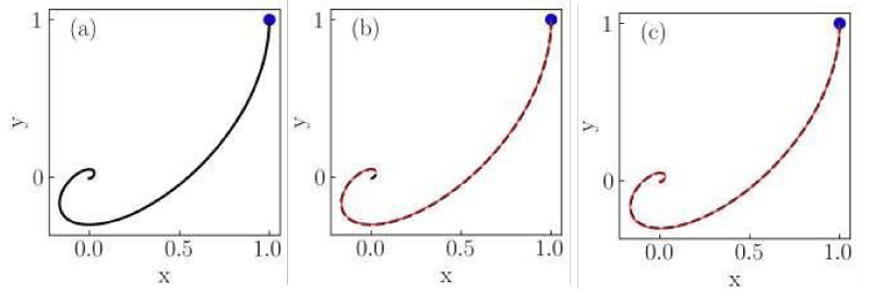
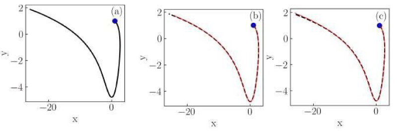
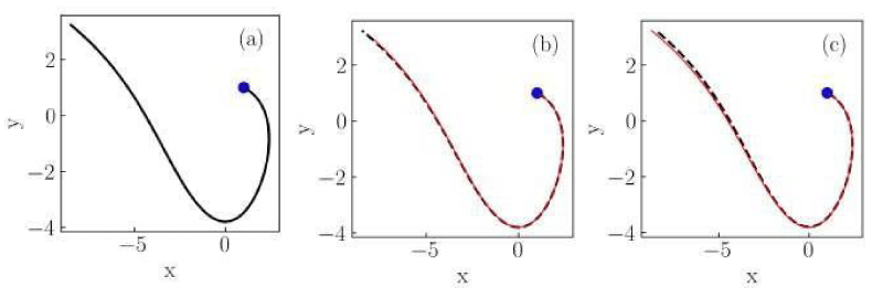
Taking into account Definition 1, we consider the generalized Liénard type system of (9). We must point out that the two-dimensional systems presented below are studied under classical ordinary operators. The interesting thing about our study is that they are considered under new local generalized differential operators, both conformable and non-conformable. All this is possible, given the generality and breadth of the operator of Definition 1, since it allows "varying" both the kernel itself and the order of the considered operator. The classical case (obtained when F ≡ 1) is added as a reference for the reader and that supports our conclusions.

We can also point out two additional details. First, given the intention of showing different variations of the system (9), we have consulted various sources dating back 30 years, they are results established as starting points for various subsequent investigations, and second, we could consider two large classes of systems presented, those that satisfy the Theorems indicated above and those that do not satisfy some of the stated considerations and the reason is the following: both classes are "good" in the following sense: they are asymptotically stable or unstable. This allows us to affirm that both behaviors continue to be maintained in the generalized case.

Case I

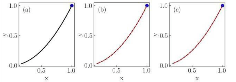
The conditions of Theorem 13 are satisfied ([34,35]) (Figures 1,2).

$\{\begin{array}{ll}{N}_T^{\alpha }x\mathrm{<mo>=</mo>}y-\left(x^3+x\right)\mathrm{,}\hfill & \hfill \\ N_T^{\alpha }y\mathrm{<mo>=</mo>}-x\mathrm{,}\hfill & \hfill \end{array}\text{ (10)}$

Case II

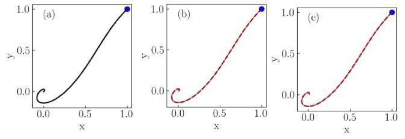
The conditions of Theorem 13 hold, with λ=1 (adapted from [36]) (Figures 3,4).

$\{\begin{array}{ll}{N}_T^{\alpha }x\mathrm{<mo>=</mo>}y-\left(\frac{x^3}{3}-x\right)\mathrm{,}\hfill & \hfill \\ N_T^{\alpha }y\mathrm{<mo>=</mo>}-x\left[1+\frac{x^2\mathrm{<mo\; stretchy="false">(</mo>}{x}^2-\mathrm{4<mo\; stretchy="false">)</mo>}}{16}\right]\mathrm{,}\hfill & \hfill \end{array}\text{ (11)}$

Case III

The function F does not satisfy the conditions of Theorem 13 so there are solutions that cannot be extended to the future (see [37,38]) (Figures 5,6).

$\{\begin{array}{ll}{N}_T^{\alpha }x\mathrm{<mo>=</mo>}y-\left(\frac{3x^2}{2}-x\right)\mathrm{,}\hfill & \hfill \\ N_T^{\alpha }y\mathrm{<mo>=</mo>}-x^3\mathrm{,}\hfill & \hfill \end{array}\text{ (12)}$

Case IV

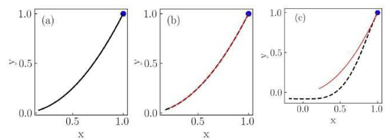
In this case, there is no λ>0 such that $g\mathrm{<mo\; stretchy="false">(</mo>}x\mathrm{<mo\; stretchy="false">)</mo>}F\mathrm{<mo\; stretchy="false">(</mo>}x\mathrm{<mo\; stretchy="false">)</mo>}\ge -\lambda$ . As in the previous case, there are solutions that cannot be extended ([39]).

$\{\begin{array}{ll}{N}_T^{\alpha }x\mathrm{<mo>=</mo>}y+\sqrt{2}{x}^2\mathrm{,}\hfill & \hfill \\ N_T^{\alpha }y\mathrm{<mo>=</mo>}-x^3\mathrm{,}\hfill & \hfill \end{array}\text{ (13)}$

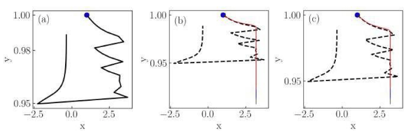
Remark: The same graph did not appear. We have the following for the common case, with time steps dt = 0.001 and total time t = 0.3:

Some variations were obtained without square root and F(x)=-x² and g(x)=-x³, with step dt0.01 and total time t = 3:

We also "approximate" the value of the root by considering $F\mathrm{<mo\; stretchy="false">(</mo>}x\mathrm{<mo\; stretchy="false">)</mo><mo>=</mo>}-\mathrm{<mo\; stretchy="false">(</mo>}{x}^2\mathrm{<mo\; stretchy="false">)</mo><mo\; stretchy="false">(</mo>0.99}\sqrt{2}\mathrm{<mo\; stretchy="false">)</mo>}$ and g(x)=-x³, with step dt = 0.001 and total time t = 8, obtaining:

Case V

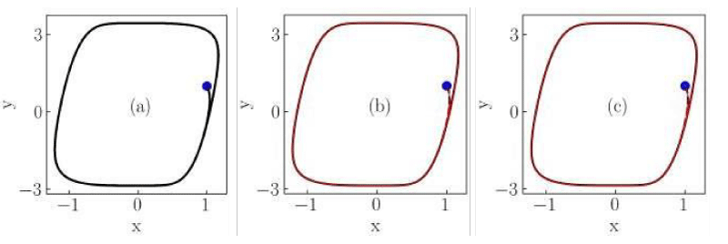
In ([40]), the following system with a limit cycle was studied (Figures 7,8).

$\{\begin{array}{ll}{N}_T^{\alpha }x\mathrm{<mo>=</mo>}y-x\mathrm{<mo\; stretchy="false">(</mo>}x-\mathrm{1<mo\; stretchy="false">)</mo><mo\; stretchy="false">(</mo>}x+\mathrm{1.1<mo\; stretchy="false">)</mo>,}\hfill & \hfill \\ N_T^{\alpha }y\mathrm{<mo>=</mo>}-x^3\mathrm{,}\hfill & \hfill \end{array}\text{ (14)}$

Case VI

The following lineal case can be studied as the limiting case of the equation 2, with F = 1 and g(x)=x. That is, it satisfies all the conditions of the Theorem 13 (Figures 9,10).

$\{\begin{array}{ll}{N}_T^{\alpha }x\mathrm{<mo>=</mo>}y-x\mathrm{,}\hfill & \hfill \\ N_T^{\alpha }y\mathrm{<mo>=</mo>}-x\mathrm{,}\hfill & \hfill \end{array}\text{ (15)}$

Variations

Below we present a group of known results from the literature, which illustrate the previous conclusions. It is not difficult to verify that if the conditions of Theorem 13 are satisfied, all solutions can be extended to the future and if those related to the function F are not met, there are unbounded solutions in finite time (Figures 11,12).

Example 16 [41]

$\{\begin{array}{ll}{N}_T^{\alpha }x\mathrm{<mo>=</mo>}y-\left(x+\frac{x^3}{3}\right)\mathrm{,}\hfill & \hfill \\ N_T^{\alpha }y\mathrm{<mo>=</mo>}-x^3\mathrm{,}\hfill & \hfill \end{array}\text{ (16)}$

Example 17 [42]

$\{\begin{array}{ll}{N}_T^{\alpha }x\mathrm{<mo>=</mo>}my-\left(-3\sqrt{m}x+2.2\sqrt{m}si{n}^{2}x\right)\mathrm{,}\hfill & \hfill \\ N_T^{\alpha }y\mathrm{<mo>=</mo>}-x\mathrm{,}\hfill & \hfill \end{array}\text{ (17)}$

$m\mathrm{<mo>></mo>0}$

Observations: Both the value of m and t make the curves grow very quickly. So much so that the values m = 0.05 and 1

Example 18 [42]

$\{\begin{array}{ll}{N}_T^{\alpha }x\mathrm{<mo>=</mo>}my-\left(-k\sqrt{m}x+l\sqrt{m}si{n}^{2}x\right)\mathrm{,}\hfill & \hfill \\ N_T^{\alpha }y\mathrm{<mo>=</mo>}-x\mathrm{,}\hfill & \hfill \end{array}\text{ (18)}$

$m\mathrm{<mo>></mo>0},k+\frac{l}{2}\mathrm{<mo>></mo>2}$

In the following figures 18 was graphed with the values m = 2, k = 9/20, I = 6 (Figures 15,16)

Example 19 [43]

$\{\begin{array}{ll}{N}_T^{\alpha }x\mathrm{<mo>=</mo>}y-k\mathrm{<mo\; stretchy="false">(</mo>}x+\frac{5}{2}\mathrm{<mo\; stretchy="false">)</mo><mo\; stretchy="false">(</mo>}x-\mathrm{3<mo\; stretchy="false">)</mo>,}\hfill & \hfill \\ N_T^{\alpha }y\mathrm{<mo>=</mo>}-x\mathrm{,}\hfill & \hfill \end{array}\text{ (19)}$

$k\mathrm{<mo>=</mo>}\frac{9}{20}\mathrm{,}\frac{7}{25}$

18 was graphed with the values k = 9/20 (Figures 17,18)

18 was graphed with the values k = 7/25 (Figures 19,20)

Example 20 [43] (Figures 21,22)

$\{\begin{array}{ll}{N}_T^{\alpha }x\mathrm{<mo>=</mo>}y-\sqrt{3}x\mathrm{<mo\; stretchy="false">(</mo>}x+\mathrm{1<mo\; stretchy="false">)</mo><mo\; stretchy="false">(</mo>}x-\mathrm{3<mo\; stretchy="false">)</mo>,}\hfill & \hfill \\ N_T^{\alpha }y\mathrm{<mo>=</mo>}-x\mathrm{,}\hfill & \hfill \end{array}\text{ (20)}$

Example 21 [43]

$\{\begin{array}{ll}{N}_T^{\alpha }x\mathrm{<mo>=</mo>}y-\lambda \left(\frac{64}{35\pi }{x}^7-\frac{112}{5\pi }{x}^5+\frac{196}{3\pi }{x}^3-\frac{C}{2}{x}^2-\frac{36}{\pi }x\right)\mathrm{,}\hfill & \hfill \\ N_T^{\alpha }y\mathrm{<mo>=</mo>}-x\mathrm{,}\hfill & \hfill \end{array}\text{ (21)}$

C =47, λ ≥ 2.86896 and λ ≥ 0.862

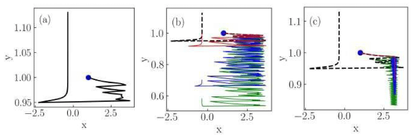
Observations: 1) For all the following cases (ordinary, conformable, and non-conformable) λ = 4.5 was considered.

2) For the common curve (black dotted line) steps of dt = 0.001 and a final time of tf = 0.5 were considered.

3) For the second conformable case in (c) with $F\mathrm{<mo\; stretchy="false">(</mo>}t\mathrm{,}\alpha \mathrm{<mo\; stretchy="false">)</mo>}\mathrm{<mo>=</mo>}{e}^{\mathrm{<mo\; stretchy="false">(</mo>1}-\alpha \mathrm{<mo\; stretchy="false">)</mo>}t}$ , even with small steps and maximum execution time of the program (it was considered dt = 0.00001 and tf = 0.001, respectively) it was observed that the values of y were increasingly negative (the value y = -75 was reached for x =). Therefore, it can be assumed that they did not achieve the same behavior as in case (b). In fact, for these same values, it can be observed that with parameter α=0.9 the curve is ``faster" (green curve), than with α=0.925 (blue curve) and with α=0.975 (red curve). For the following graphs, it was decided to maintain the step values dt = 0.00001 and maximum execution time tf = 0.0001 for the red, blue, and green curves.

4) For the conformable case in (b) with $F\mathrm{<mo\; stretchy="false">(</mo>}t\mathrm{,}\alpha \mathrm{<mo\; stretchy="false">)</mo>}\mathrm{<mo>=</mo>}{t}^{\mathrm{<mo\; stretchy="false">(</mo>1}-\alpha \mathrm{<mo\; stretchy="false">)</mo>}}$ it was enough to consider steps of dt = 0.001 and a final time of tf = 0.5 to see the graphs below.

5) For the non-conformable case in (b) with $F\mathrm{<mo\; stretchy="false">(</mo>}t\mathrm{,}\alpha \mathrm{<mo\; stretchy="false">)</mo>}\mathrm{<mo>=</mo>}{e}^{t^{-\alpha }}$ the steps of dt = 0.001 and a final time of tf = 0.55 and in (c) with $F\mathrm{<mo\; stretchy="false">(</mo>}t\mathrm{,}\alpha \mathrm{<mo\; stretchy="false">)</mo>}\mathrm{<mo>=</mo>}{t}^{\alpha }$ the steps of dt = 0.001 and a final time of tf = 0.2 (Figures 23,24) .

In addition to (Figures 19, 25,26)[15]

$\{\begin{array}{ll}{N}_T^{\alpha }x\mathrm{<mo>=</mo>}my-\left(-k\sqrt{m}x+lx\sqrt{m}si{n}^{2}x\right)\mathrm{,}\hfill & \hfill \\ N_T^{\alpha }y\mathrm{<mo>=</mo>}-x\mathrm{,}\hfill & \hfill \end{array}\text{ (22)}$

$m\mathrm{<mo>></mo>0},k+\frac{l}{2}\mathrm{<mo>></mo>2}$

Conclusion

In this work, we have presented a set of examples, known from the literature, in which the following conclusion can be seen: The study of the equilibrium points of the ordinary system provides clues to the behavior of the system under other differential operators. What does this mean for an applied researcher or an area related to the physical sciences? It means that the study of a generalized model must be accompanied by the qualitative study of the corresponding ordinary system. In fact, the previous analysis of the corresponding ordinary system can considerably help the understanding of the simulation of a system under generalized differential operators.

1. Liapounov AM. Problème général de la stabilité du mouvement, in Annals of Math. Studies No.17, Princeton Univ. Press, Princeton, NJ. 1949.
2. H. A. A survey of Lyapunov's second method contributions to the theory of nonlinear oscillations IV in Annals of Math. Studies No.44, Princeton Univ. Press, Princeton, NJ. 1958.
3.  Barbashin EA. Liapunov's Functions, Science Publishers, Moscow. 1970 (Russian).
4. Cesari L. Asymptotic behavior and stability problems in ordinary differential equations, Springer-Verlag, Berlin. 1959.
5. Demidovich BP. Lectures on the Mathematical Theory of the Stability, Science Publishers, Moscow. 1967. (Russian).
6. Hahn W. Theory and Application of Liapunov's Direct Method, Prentice-Hall, Englewood Cliffs. New Jersey. 1963.
7. Yoshizawa T. Stability theory by Liapunov's second method. The Mathematical Society of Japan. 1966.
8. Nápoles JEV. A continuation result for a bi-dimensional system of differential equation. Revista Integración. 1995; 13(2): 49-54.
9. Hale K, Hara T, Yoneyama T, Sugie J. Necessary and Sufficient Conditions for the Continuability of Solutions of the System x'=y-F(x), y'=-g(x), Applicable Analysis: An International Journal. 1985; 19: 169-180.
10. Hasan YQ, Zhu LM. The bounded solutions of Liénard equation, J. of Applied Sciences. 2007; 7(8): 1239-1240.
11. Helms LL. Introduction To Potential Theory (New York: Wiley-Interscience. 1969.
12. LaSalle JP. Some extensions of Liapunov's second method. IRE Transaction on Circuit Theory. 1960; 520-527.
13. Lugo LM, Nápoles JEV, Noya SI. On the construction of regions of stability. Pure and Applied Mathematics Journal. 2014; 3(4): 87-91.
14. Nápoles JEV. On the continuability of solutions of bidimensional systems. Extracta Mathematicae. 1996; 11(2): 366-368.
15. Nápoles JEV. On the boundedness and asymptotic stability in the whole of Liénard equation with restoring term. Revista de la Unión Matemática Argentina. 2000; 41(4): 47-59. (Spanish).
16. Peng L, Huang L. On global asymptotic stability of the zero solution of a generalized Lienard's system. Appl. Math-JCU. 1994; 9B: 359-363.
17. Liénard A. Étude des oscillations entretenues.
18. Van BDP. On oscillation hysteresis in a triode generator with two degrees of freedom. Phil. Mag. 1922; (6) 43: 700–719.
19. Van BDP. On `relaxation-oscillations'. Philosophical Magazine. 1926; 2(11):978-992.
20. Machado JT, Kiryakova V, Mainardi F. Recent history of fractional calculus. Commun. Nonlinear Sci. Numer. Simul. 2011; 16: 1140-1153.
21. Nápoles JEV. The non-integer local order calculus. Phys Astron Int J. 2023; 7(3):163-168. DOI: 10.15406/paij.2023.07.00304
22. Guzmán PM, Lugo LM, Nápoles VJE, Vivas M. On a New Generalized Integral Operator and Certain Operating Properties. Axioms. 2020; 9: 69. doi:10.3390/axioms9020069.
23. Nápoles JE, Guzmán PM, Lugo LM, Kashuri A. The local nonconformable derivative, and Mittag Leffler function. Sigma J Eng & Nat Sci. 2020; 38 (2): 1007-1017.
24. Zhao D, Luo M. General conformable fractional derivative and its physical interpretation. Calcolo. 2017; 54: 903-917. DOI 10.1007/s10092-017-0213-8.
25. Fleitas A, Nápoles VJE, Rodr JM. guez JM. Sigarreta, NOTE ON THE GENERALIZED CONFORMABLE DERIVATIVE, Revista de la UMA. 2021; 62: 2; 443-457. https://doi.org/10.33044/revuma.1930
26. Guzmán PM, Langton G, Lugo LM, Medina J, Nápoles VJE. A new definition of a fractional derivative of local type, J. Math. Anal. 2018; 9:2; 88-98.
27. Nápoles JEV, Guzmán PM, Lugo LM. Some New Results on Nonconformable Fractional Calculus, Advances in Dynamical Systems and Applications ISSN 0973-5321. 2018; 13: 2; 167-175.
28. Fleitas A,Méndez JA, Nápoles JE, Sigarreta JM. On the some classical systems of Liénard in general context, Revista Mexicana de Física. 2019; 65 (6): 618-625.
29. Khalil R, Horani MAl, Yousef A, Sababheh M. A new definition of fractional derivative. J. Comput. Appl. Math. 2014; 264: 65-70.
30. Nápoles JEV, Rodr JM, guez JM. Sigarreta, On Hermite-Hadamard type inequalities for non-conformable integral operators, Symmetry 2019; 11: 1108. doi:10.3390/sym11091108.
31. Martínez F, Mohammed PO, Nápoles JEV. Non Conformable Fractional Laplace Transform, Kragujevac. Journal of Mathematics. 2022; 46(3): 341-354.
32. George EC, Juan E. Nápoles Valdés, Continuability of Liénard's Type System with Generalized Local Derivative, Discontinuity, Nonlinearity, and Complexity. 2023; 12(1): 1-11. DOI:10.5890/DNC.2023.03.001
33. Huang Lih, Bin-Xiang Dai, Si-hu Hu. Continuability of Solutions for a Generalized Liénard System. J. of Hunan University. 1999; 26(6): 1-9.
34. Nápoles JEV. On the global stability of non-autonomous systems. Revista Colombiana de Matemáticas. 1999; 33: 1-8.
35. Nápoles JEV, Repilado JAR. On the boundedness and stability in global sense of the solutions of a two-dimensional system of differential equations, Revista Ciencias Matemáticas. 1997; XVI: 71-74.
36. Odani K. The limit cycle of the Vanderpol equation is not algebraic. Journal of Differential Equations. 1995; 115: 146-152.
37. Hricisákova D. Continuability and (non-)oscillatory properties of solutions of generalized Liénard equation. Hiroshima Math. J. 1990; 20: 11-22.
38. Hricisákova D. Negative solutions of the generalized Lienard equation. Hiroshima Mathematical Journal. 1992; 23: 155-160.
39. Yu SX, Zhang JZ. On the center of the Li´enard equation. Journal of Differential Equations. 1993; 102: 53-61.
40. Kooij RE, Jianhua S. A note on uniqueness of limit cycles in Liénard type systems, J. Math. Anal. Appl. 1997; 208: 260-276.
41. Yu SX, Zhang JZ. On the center of the Li´enard equation. Journal of Differential Equations. 1993; 102: 53-61.
42. Aghajani A, Moradifam A. The Generalised Lienard Equations. Glasgow Math. J. 2009; 51: 605-617. doi:10.1017/S0017089509990036
43. Hayashi M, Villari G, Zanolin F. On the uniqueness of limit cycle for certain Liénardsystems without symmetry, Electronic. Journal of Qualitative Theory of Differential Equations. 2018; 1-10. https://doi.org/10.14232/ejqtde.2018.1.XX
44. Guzmán PM, Luciano M. Lugo Motta Bittencurt, Juan E. Nápoles Valdes, A Note on Stability of Certain Liénard Fractional Equation, International Journal of Mathematics and Computer Science. 2019; 14: 2; 301-315.